Book TOC · Previous · Chapter 3 of 7 · Next

Chapter 3: Scaling Prototypes into Models: Custom Training, Fine-Tuning (PEFT/LoRA) & Hardware Accelerators

Subsections Covered: 3.1, 3.2, 3.3 (12 Considerations · 24 Custom Visual Diagrams)

Chapter Focus: Explainable AI (Shapley/Integrated Gradients), custom training containers, Vertex AI Vizier hyperparameter tuning, LoRA/RLHF fine-tuning vs. RAG, CPU/GPU/TPU selection, and Data vs. Model Parallelism (MultiWorkerMirroredStrategy, TPUStrategy).

Subsection 3.1: Building models given the task considering cost, complexity, latency, and scalability

Section 3: Scaling prototypes into ML models

The Big Picture

When scaling an ML prototype into production, a common failure mode is Architectural Overkill: choosing a 70-billion-parameter LLM or a deep neural network when a gradient-boosted decision tree (XGBoost) or ARIMA_PLUS solves the problem at $1/50\text{th}$ the cost and latency—or choosing a black-box deep network when regulators demand an intrinsically interpretable white-box model. Subsection 3.1 tests your ability to balance four competing forces across every modeling decision:

1. Choosing the Right Model Family for Data Modality & Sample Size (3.1a):
2. Structured/tabular data with medium scale and CPU budget → Gradient Boosted Decision Trees (XGBoost / LightGBM) or Linear/Logistic Models.
3. Univariate/multi-series time forecasting → ARIMA_PLUS; complex multi-covariate tabular forecasting → Temporal Fusion Transformers / AutoML Forecasting.
4. Small labeled image dataset (e.g., 500 rare medical images) → Transfer Learning (freezing pre-trained CNN/ViT backbone weights and training a lightweight classification head) with Data Augmentation rather than training a deep CNN from scratch (which severely overfits).
5. Choosing the Right Google Cloud Product (3.1b): Matching team skill and control requirements along the Buy → Low-Code → Custom spectrum (Prebuilt API → BigQuery ML → Agent Platform AutoML → Custom Training / Pipelines).
6. Choosing the Right Deployment & Serving Strategy (3.1c):
7. Offline/disconnected mobile or IoT devices → Lightweight architecture (MobileNet / quantized model) compiled to LiteRT (TensorFlow Lite) on-device.
8. Static reference features with strict <5ms global latency (e.g., homepage movie recommendations computed nightly) → Batch pre-computation written to Cloud Bigtable or Memorystore rather than running live GPU inference on every page load.
9. Dynamic context-dependent features requiring immediate response → Synchronous Online Prediction on Agent Platform Endpoints.
10. Satisfying Interpretability & Regularization Requirements (3.1d): Distinguishing Intrinsic ("White-Box") Interpretability (Linear/Logistic Regression, GAMs, shallow Decision Trees where mathematical coefficients directly define the decision boundary) from Post-Hoc Attribution (Vertex Explainable AI: Sampled Shapley for trees, Integrated Gradients for DNNs, XRAI for images), while controlling model complexity via $L_1$ (Lasso), $L_2$ (Ridge), Dropout, Batch Normalization, and Early Stopping.

Consideration 3.1a: Choosing the model type (e.g., ARIMA, DNN, and LLM)

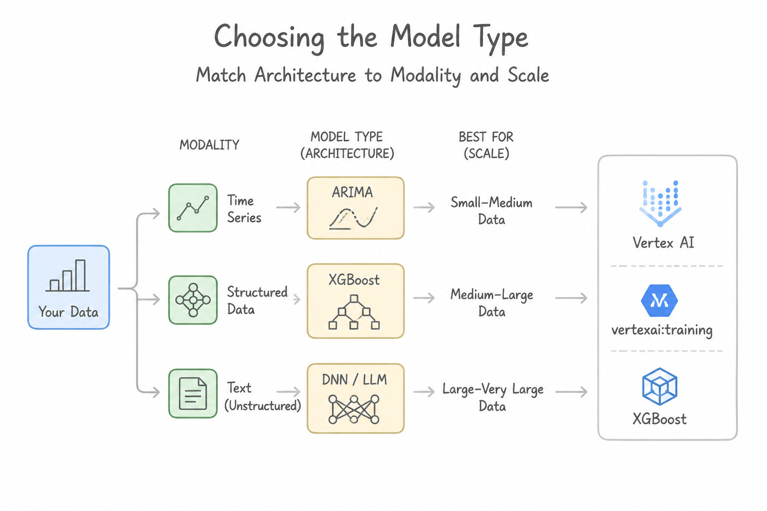
• Matching Model Architecture to Modality & Scale:
• Structured / Tabular Data: Gradient Boosted Decision Trees (XGBoost) train rapidly on CPUs, handle mixed feature scales naturally, and consistently match or beat deep neural networks on medium-sized tabular datasets at a fraction of the compute cost.
• Time-Series Data: Use ARIMA_PLUS for classical statistical trend/seasonality decomposition; use Deep Neural Networks (DNNs / RNNs / Transformers) when modeling complex high-dimensional cross-series interactions.
• Scarce Labeled Data (e.g., 500 medical images): Never train a deep CNN or Vision Transformer from random initialization on a tiny dataset—it will memorize the training set. Use Transfer Learning: load a backbone pre-trained on a massive dataset (e.g., ImageNet / Model Garden), freeze the early feature-extraction layers, and train only the top classification head alongside Data Augmentation.
• Standard Loss Functions & Optimizers:
• Multi-Class Classification: Categorical Cross-Entropy Loss (paired with a Softmax output layer).
• Linear Regression: Mean Squared Error (MSE) or Huber/MAE loss.
• Adaptive Optimizers: Adam (Adaptive Moment Estimation) dynamically adjusts per-parameter learning rates using running averages of first and second moments of the gradients; for deep RNNs/Transformers, apply Gradient Clipping and residual/gated connections (LSTM/GRU/Attention) to prevent vanishing and exploding gradients.
• Diagnosing & Fixing Overfitting vs. Underfitting:
• Overfitting Signal: Training loss continues to drop toward zero while validation loss diverges and increases. Remediation: Apply Early Stopping, $L_2$ (Ridge) regularization (penalizes squared weights $\lambda \sum w_i^2), **@@CODE₁@@ (Lasso) regularization (penalizes absolute weights \lambda \sum |w_i|, driving unimportant feature weights to exact zero for automatic feature selection), Dropout (randomly zeroes neuron activations during training), or Data Augmentation**.
• Underfitting Signal: Both training loss and validation loss remain high and plateau early. Remediation: Increase model capacity (more layers/units, switch from linear to DNN/XGBoost), train longer, decrease regularization (\lambda), or engineer richer domain features.

Key Implementation Patterns

• Small Dataset Image Classification: Use Use a model architecture pre-trained on a large dataset and fine-tune the final layers on your images. Transfer learning uses pre-existing knowledge from large datasets to solve tasks with limited data, preventing overfitting. (Avoid alternative: Unsupervised clustering ignores the provided labels and is not suitable for a specific classification task.)
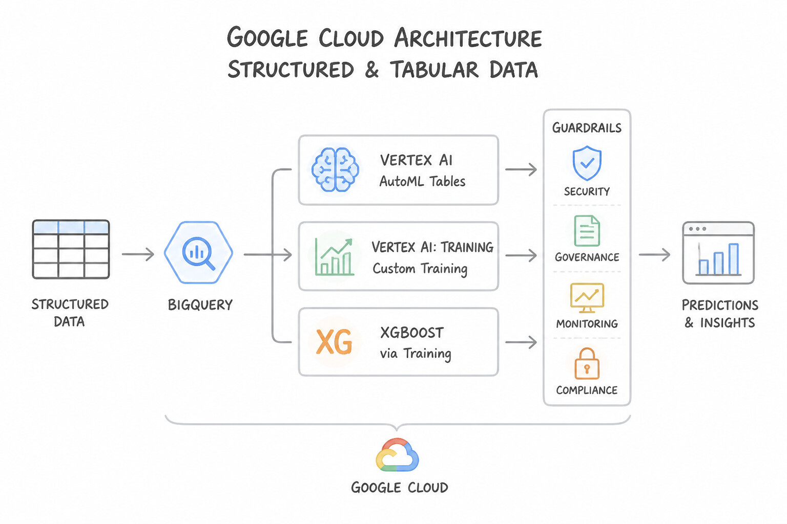
• Leveraging SQL Skills for Regression: Use Use the XGBoost framework to train a gradient boosted decision tree model. XGBoost is the preferred framework for structured/tabular data on CPUs due to its speed, efficiency, and high accuracy without extensive tuning. (Avoid alternative: RNNs are designed for sequential data and are computationally slow on CPUs compared to tree-based models for general tabular classification.)
• Predicting Continuous Values with BQML: Use Set the model_type option to LINEAR_REG. Linear Regression is the correct algorithm for predicting continuous values like sales amounts or prices. (Avoid alternative: Logistic Regression is used for classification tasks (predicting categories), not for predicting continuous numerical values.)

Key Takeaways (3.1a)

• Small Data + Complex Task = Transfer Learning: When you lack massive datasets for image or text tasks, always look for pre-trained models first.
• Avoid Training from Scratch: Training deep networks from random initialization requires thousands or millions of examples to avoid overfitting.
• Model Complexity: Increasing model size (layers/parameters) on small datasets increases overfitting.
• Use Gradient Boosted Trees (like XGBoost) for structured/tabular data problems.

Consideration 3.1b: Choosing the product (e.g., Agent Platform AutoML, BigQuery ML, and Agent Platform Pipelines)

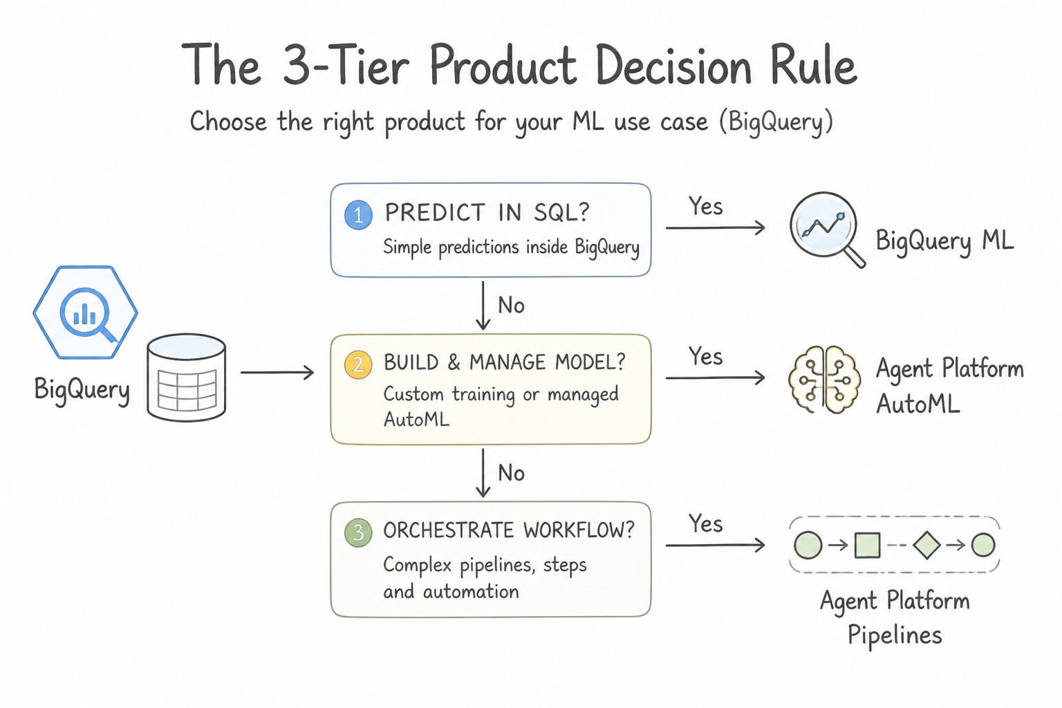
• The 3-Tier Product Decision Rule (BigQuery ML vs. Agent Platform AutoML vs. Agent Platform Custom Training / Pipelines):
• Choose BigQuery ML when the data already resides in BigQuery, the problem fits supported SQL model types (LINEAR_REG, LOGISTIC_REG, BOOSTED_TREE_*, ARIMA_PLUS, KMEANS, MATRIX_FACTORIZATION, remote Gemini), and the team consists of data analysts or wants the lowest operational overhead with zero data movement.
• Choose Agent Platform AutoML when you need maximum out-of-the-box predictive accuracy on Tabular, Forecasting, Image, Text, or Video data using custom labels, the team has limited ML engineering staff or tight launch deadlines, and you do not need to write custom neural network code.
• Choose Agent Platform Custom Training + Agent Platform Pipelines when you require full control over the model architecture (custom PyTorch/TensorFlow/JAX layers, custom loss functions), specialized C++ libraries, or automated multi-stage MLOps workflows.

Key Implementation Patterns

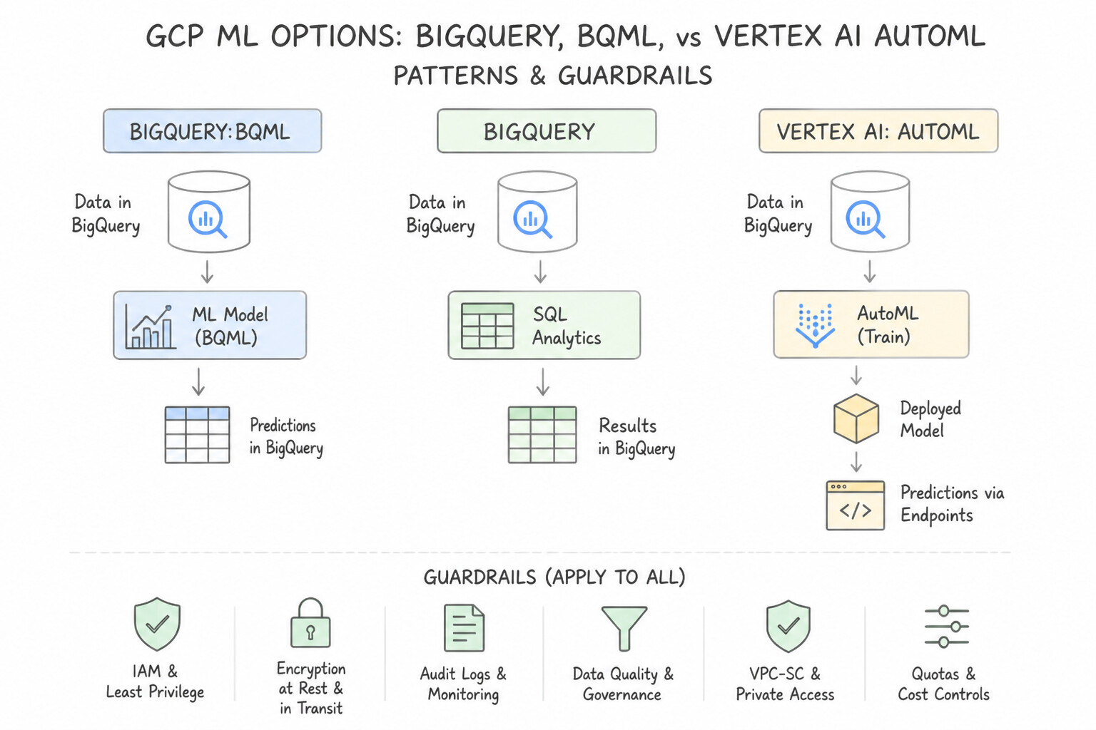
• Leveraging SQL Skills for Regression: Use Use BigQuery ML to create and train an ARIMA_PLUS forecasting model using standard SQL queries. BigQuery ML lets the team use their existing SQL skills to train models directly inside the data warehouse without moving data. (Avoid alternative: Exporting data and using TensorFlow requires Python skills the team lacks and moves data unnecessarily.)
• AutoML vs. Custom Training for Rapid Prototyping: Use Train a classification model using Vertex AI AutoML for tabular data. AutoML automates model creation for tabular data, requiring minimal code and expertise. (Avoid alternative: Kubeflow on GKE adds unnecessary operational complexity and requires high expertise.)
• Strict Regulatory Compliance: Use Run a batch prediction job and store the results in Cloud Bigtable. Configure the application to retrieve recommendations from Cloud Bigtable. Cloud Bigtable provides the required high throughput and single-digit millisecond latency for serving pre-computed data.

Key Takeaways (3.1b)

• Minimize Data Movement: For large datasets (petabytes), bring the compute to the data, not the data to the compute.
• Leverage Existing Skills: If a team is proficient in SQL, BigQuery ML is often the fastest path to production compared to retraining them in Python.
• BigQuery ML Capabilities: BQML supports regression, classification, clustering, and time-series forecasting (ARIMA_PLUS) using SQL.
• Use Vertex AI AutoML for rapid prototyping and high-quality baselines when using standard data types (tabular, image, text).

Consideration 3.1c: Choosing the deployment strategy

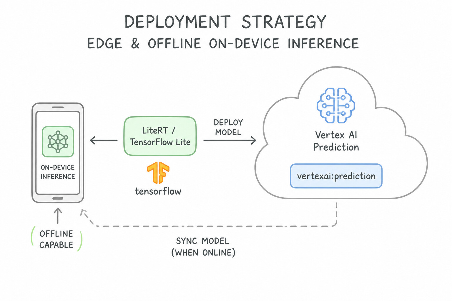
• Edge / Offline On-Device Inference (LiteRT / TensorFlow Lite): When the scenario specifies no internet connectivity (e.g., remote agricultural fields, maritime ships, factory floor sensors) or strict client-side privacy/zero-network-latency on mobile/IoT devices, select a lightweight mobile architecture (such as MobileNet or EfficientNet-Lite), quantize the weights (FP32 → INT8), and export to LiteRT (TensorFlow Lite .tflite) for on-device execution.
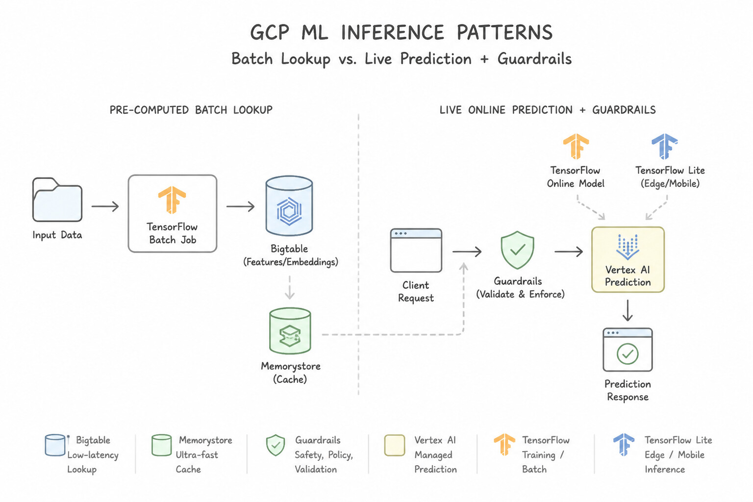
• Pre-Computed Batch Lookup (Bigtable / Memorystore) vs. Live Online Prediction:
• If predictions depend only on slow-changing or static reference features (e.g., nightly personalized movie carousels or daily customer propensity scores for 50 million users) and the web app requires single-digit millisecond latency at minimal serving cost, run a scheduled Batch Prediction job nightly and load the pre-computed top-$K$ results into Cloud Bigtable or Memorystore for Redis for instant key-value lookup.
• If predictions depend on live, dynamic request-time context (e.g., real-time credit card swipe amount, current GPS location, live chat utterance), deploy the model to an Agent Platform Online Prediction Endpoint.

Key Implementation Patterns

• Optimizing for Edge Deployment: Use Train a MobileNet model and convert it to TensorFlow Lite format. MobileNet is optimized for mobile devices, and TensorFlow Lite enables offline on-device inference. (Avoid alternative: Hosting on a VM requires internet connectivity, which is unavailable in remote areas.)
• Scikit-learn Artifact Naming Conventions: Use Deploy the model to a Vertex AI Endpoint. Vertex AI Endpoints provide online predictions with the low latency required for real-time blocking. (Avoid alternative: Batch prediction jobs have high startup latency and are meant for bulk data, not immediate responses.)

Key Takeaways (3.1c)

• No Internet (Offline): Requires on-device inference. You cannot use cloud endpoints (like Vertex AI prediction) or VMs.
• Mobile/Edge Constraints: Devices have limited battery, storage, and compute power. Use architectures designed for this, such as MobileNet.
• TensorFlow Lite: The standard format for deploying TensorFlow models to mobile and edge devices. It optimizes models for size and latency.
• Architecture Choice: Avoid heavy architectures (VGG, ResNet) for mobile apps unless absolutely necessary and if the device can handle it; prefer efficient ones like MobileNet, EfficientNet-Lite, or NASNet Mobile.

Consideration 3.1d: Modeling techniques given interpretability requirements

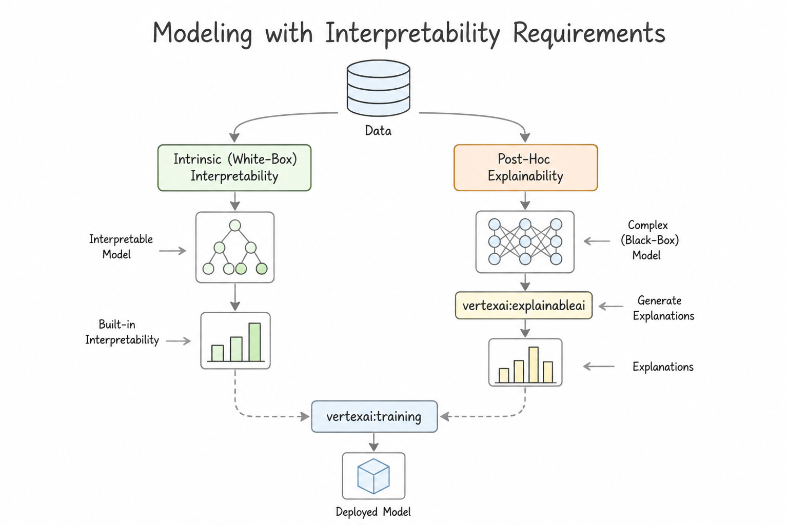
• Intrinsic ("White-Box") Interpretability vs. Post-Hoc Explainability:
• When a government agency, healthcare board, or financial regulator mandates a "white-box" or intrinsically interpretable model where stakeholders can inspect the exact global mathematical formula and monotonic feature weights directly, choose Linear Regression, Logistic Regression, Generalized Additive Models (GAMs), or shallow Decision Trees—even if a deep neural network would score 1–2% higher accuracy.
• When high accuracy on complex non-linear patterns is required alongside per-prediction local explanations (e.g., explaining why a specific loan application was declined by an XGBoost or DNN model), deploy the complex model on Agent Platform with Vertex Explainable AI enabled.
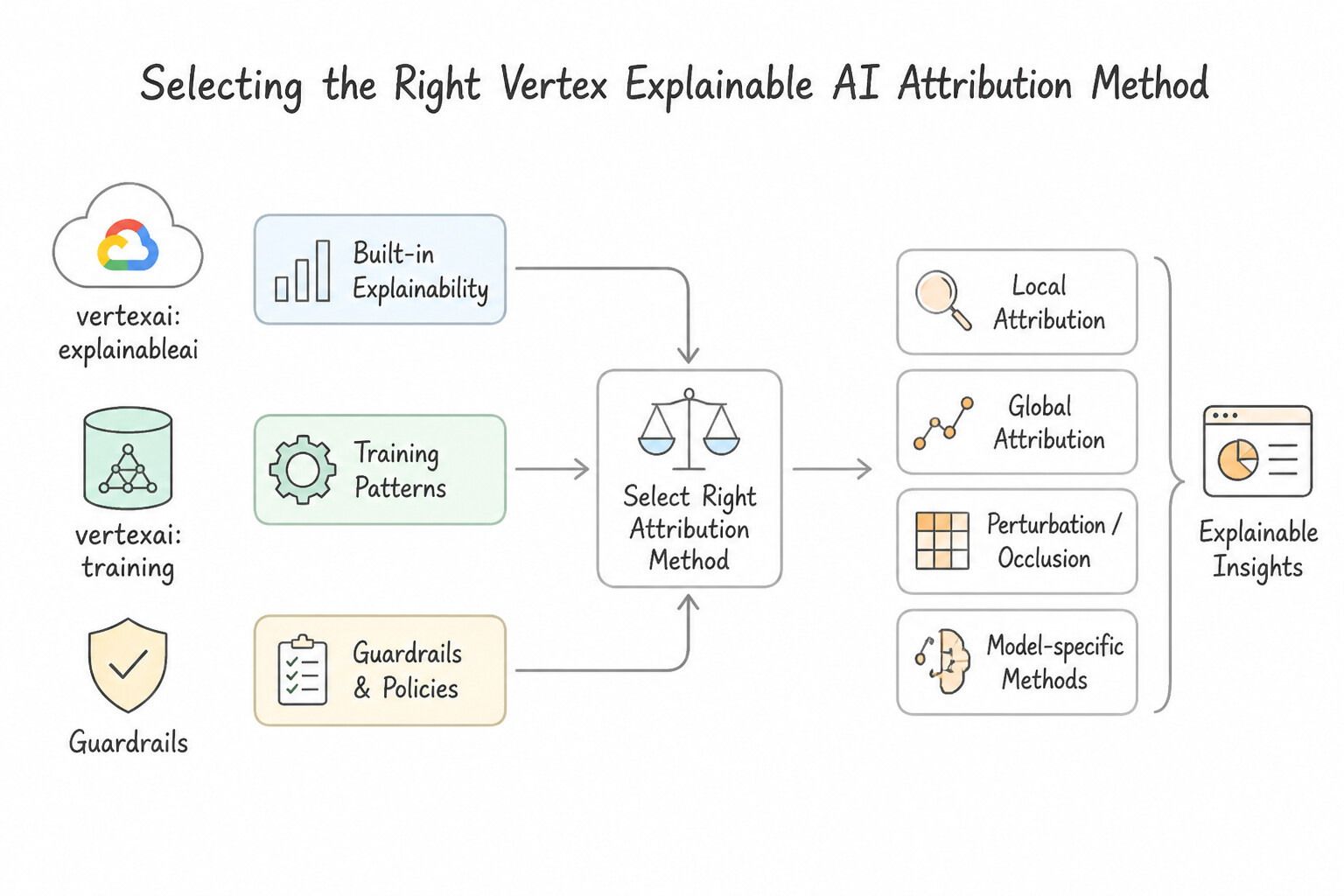
• Selecting the Right Vertex Explainable AI Attribution Method:
• Sampled Shapley: Model-agnostic cooperative game-theory approximation. Mandatory choice for non-differentiable tree-based models (XGBoost, Random Forest, Scikit-learn) on tabular data.
• Integrated Gradients: Computes path integrals of gradients along a straight line from a baseline input to the actual input. Optimal choice for differentiable neural networks (TensorFlow, PyTorch DNNs) on tabular or text data (much faster than Sampled Shapley on high-dimensional differentiable models).
• XRAI (eXplanation with Ranked Area Integrals): Combines Integrated Gradients with over-segmentation (Felzenszwalb superpixels) to highlight cohesive visual regions rather than noisy individual pixels. Optimal choice for Computer Vision / Image Classification (e.g., highlighting a fracture region on an X-ray).

Key Implementation Patterns

• Loan Approval Compliance: Use Configure Vertex AI Explainable AI to use Sampled Shapley. Sampled Shapley supports non-differentiable models like XGBoost on tabular data and provides local explanations. (Avoid alternative: Integrated Gradients is for differentiable models like neural networks, not tree-based models.)
• Medical Imaging Diagnosis: Use Configure the explanation method to use XRAI. XRAI is designed to highlight regions or segments in images, making it ideal for high-contrast X-rays. (Avoid alternative: Integrated Gradients highlights individual pixels rather than regions.)

Key Takeaways (3.1d)

• Integrated Gradients is for differentiable models (Neural Networks).
• XRAI is for Image data.
• Sampled Shapley is for non-differentiable models (Trees, Ensembles) on tabular data.
• Local explainability is required when justifying specific individual predictions.

Quick Decision Cheat Sheet (Subsection 3.1)

Further Reading (Subsection 3.1)

• Transfer learning and fine-tuning — The official TensorFlow guide explaining how to take a pre-trained model and fine-tune it for a new task, specifically addressing the benefits for small datasets.
• Vertex AI Model Garden — Documentation on Google Cloud's Model Garden, which provides access to many pre-trained models ready for transfer learning.
• XGBoost Documentation - Introduction — Provides an overview of tree boosting and its advantages for structured data.
• Tabular Data: Deep Learning is Not All You Need — A research paper comparing tree-based models and deep learning on tabular datasets, often finding trees superior for mid-sized data.
• Selection of BigQuery ML models — A guide helping users select the appropriate model type based on their use case and data.
• Vertex AI AutoML documentation — Overview of when to use AutoML versus custom training, highlighting the benefits for users with limited ML expertise.

Subsection 3.2: Training models

Section 3: Scaling prototypes into ML models

The Big Picture

Moving from a single-GPU prototype to a production training pipeline on Gemini Enterprise Agent Platform (Vertex AI Training) exposes bottlenecks across data ingestion, container packaging, failure recovery, hyperparameter search, and foundation model tuning:

1. The I/O Starvation & Redundant Export Trap (3.2a & 3.2b): Reading millions of individual JPEG or CSV files from Cloud Storage leaves expensive A100/H100 GPUs sitting at 25% utilization while CPUs wait on network I/O. Conversely, exporting a 20 TB BigQuery table to CSV files in Cloud Storage before starting a TensorFlow job adds hours of brittle ETL and storage duplication when the BigQuery Storage Read API (tensorflow-io / BigQueryClient) streams Arrow records directly into training workers.
2. Choosing the Wrong Training SDK or Container Packaging (3.2c): Using prebuilt containers when the training code depends on custom C++ bioinformatics libraries (Custom Container required), or writing proprietary cloud-locked scripts when a hybrid enterprise mandates identical pipeline execution across on-premises Kubernetes and Google Cloud (Kubeflow on GKE).
3. Training Failures: OOM, Exploding Gradients & Preemption Loss (3.2d):
4. GPU ResourceExhaustedError (OOM): Reducing batch size blindly hurts gradient stability unless paired with Gradient Accumulation or Mixed Precision (FP16/BF16).
5. NaN Loss after 200 steps in an RNN/Transformer: Caused by exploding gradients or an excessively high learning rate (fix: Gradient Clipping (clipnorm / clipvalue), Linear Warmup + Cosine Decay schedule, and checking for NaN/Inf in input data).
6. Spot / Preemptible VM eviction: Losing 18 hours of training progress because the script didn't save periodic Model Checkpoints to a durable Cloud Storage path (AIP_CHECKPOINT_DIR).
7. Brute-Force Hyperparameter Tuning & Misused Foundation Model Tuning (3.2e & 3.2f): Using Grid Search across 8 hyperparameters or tuning learning rate [0.0001, 0.1] on a linear scale instead of Bayesian Optimization with UNIT_LOG_SCALE and Median Automated Early Stopping. And for foundation models, knowing when to use Supervised Fine-Tuning (SFT) (JSONL input_text/output_text or messages), PEFT/LoRA, or RLHF (aligning conversational tone with human preference pairs).

Consideration 3.2a: Organizing training data (e.g., tabular, text, speech, images, and videos) on Google Cloud (e.g., Cloud Storage and BigQuery)

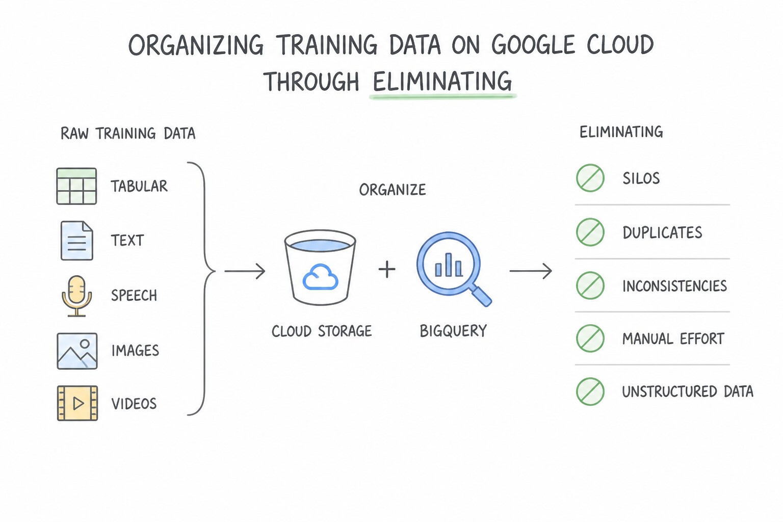
• Eliminating Small-File Overhead on Cloud Storage (TFRecord): Cloud Storage delivers massive aggregate throughput on large sequential reads (100–200 MB objects), but incurs per-object HTTP metadata latency when opening millions of tiny 20 KB JPEG or JSON files. Always pack small unstructured training files into TFRecord shards (or WebDataset .tar shards for PyTorch).
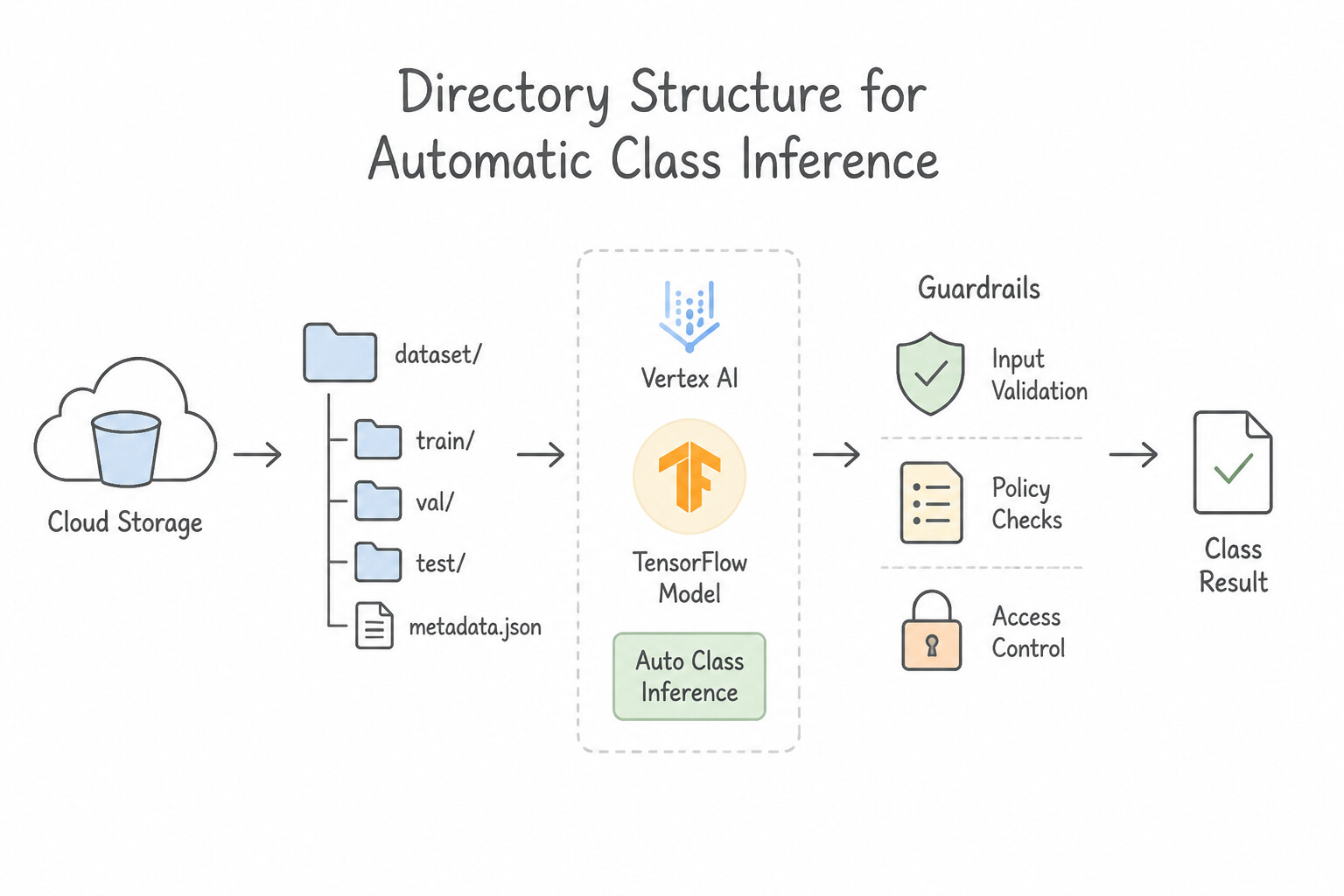
• Directory Structure for Automatic Class Inference: When using standard framework loaders like tf.keras.utils.image_dataset_from_directory or torchvision.datasets.ImageFolder on Cloud Storage Fuse (/gcs/...), organize single-label images using the canonical hierarchy: gs://bucket/train/class_a/img01.jpg, gs://bucket/train/class_b/img02.jpg.
• Direct Streaming from BigQuery for Tabular Training: When petabytes of structured training features live in BigQuery, do not export temporary CSV files to Cloud Storage. Use the BigQuery Storage Read API (via tensorflow-io's BigQueryClient or google-cloud-bigquery-storage in PyTorch/Spark) to read multiple data streams in parallel directly into worker memory.

Key Implementation Patterns

• Optimizing I/O for Large Image Datasets: Use Serialize and aggregate the images into larger container files, such as TFRecord, of approximately 100 MB each. Aggregating small files into larger container files reduces API overhead and enables efficient sequential reads. (Avoid alternative: Reducing individual file size does not address the overhead of opening millions of individual network connections.)
• Tabular Data Integration via BigQuery: Use Configure the training job to read data directly using the BigQuery Storage API. The BigQuery Storage API allows direct, high-throughput streaming of data into TensorFlow, avoiding the need for intermediate exports. (Avoid alternative: Creating TFRecord files on Cloud Storage still constitutes an export step, which the scenario aims to avoid.)
• Directory Structure for Custom Classification: Use Create a separate folder for each class label and upload the images into their corresponding folders. Standard ML frameworks use the folder name as the class label when loading images from directories. (Avoid alternative: Standard loaders usually look for folder names, not filename prefixes, to determine class labels.)

Key Takeaways (3.2a)

• Cloud Storage throughput is optimized for larger files; millions of small files cause high API overhead.
• Always aggregate small training samples (images, text) into larger container formats like TFRecord or Parquet.
• Target file sizes of roughly 100 MB to 200 MB to enable efficient sequential reads and prefetching.
• Monitor accelerator utilization (GPU/TPU duty cycle) to detect I/O bottlenecks.

Consideration 3.2b: Ingesting structured and unstructured data from various sources into training pipelines

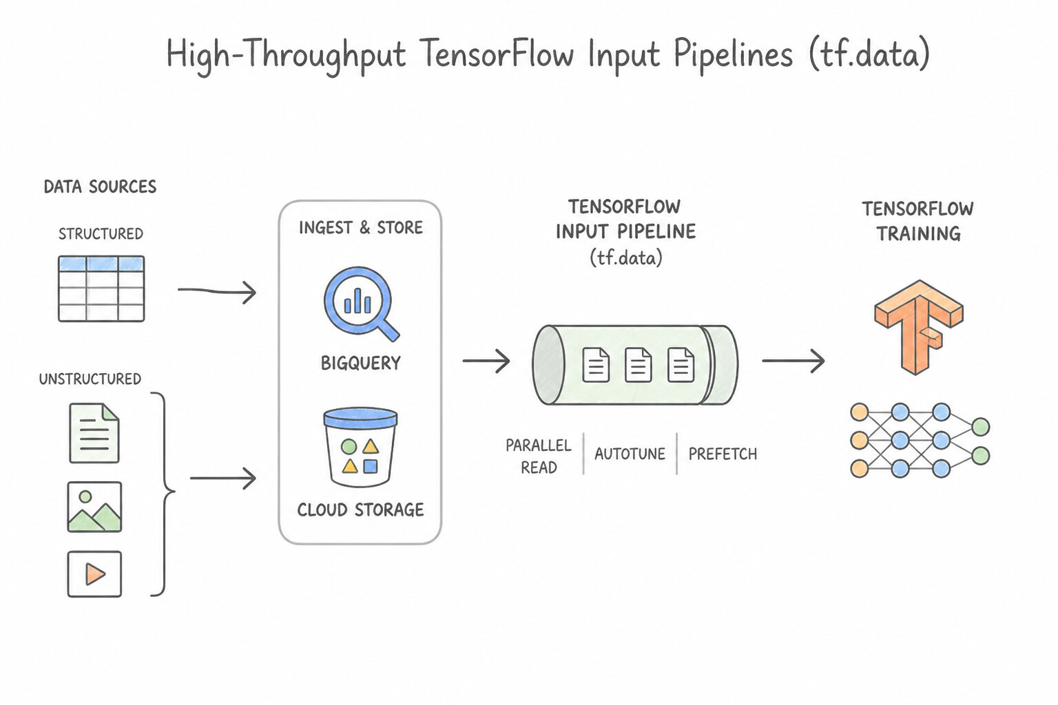
• High-Throughput TensorFlow Input Pipelines (tf.data):
• For hundreds of large CSV files in Cloud Storage, use tf.data.experimental.make_csv_dataset (which handles header parsing, column type inference, batching, and shuffling automatically) or convert to TFRecord and read with tf.data.TFRecordDataset using num_parallel_reads=tf.data.AUTOTUNE.
• Always overlap CPU data preprocessing ($N+1) with GPU/TPU forward/backward execution (@@CODE₁@@) by chaining .prefetch(tf.data.AUTOTUNE) at the end of the tf.data.Dataset pipeline, and use .interleave() + .map(..., num_parallel_calls=tf.data.AUTOTUNE).
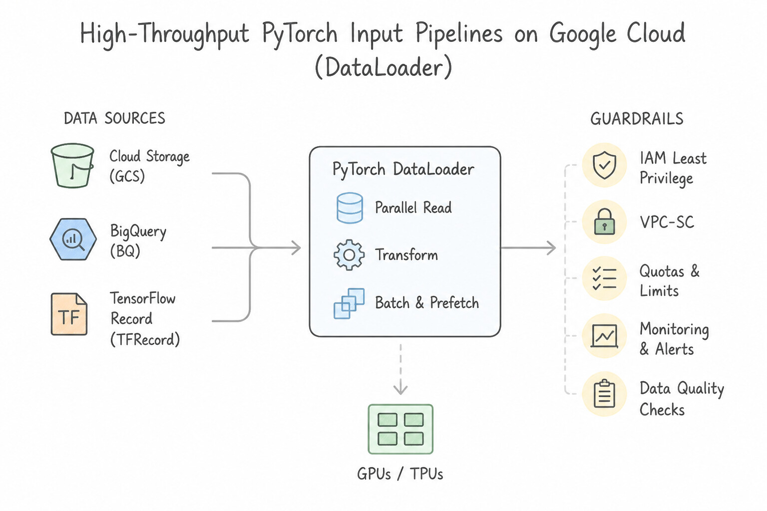
• High-Throughput PyTorch Input Pipelines (DataLoader): Configure torch.utils.data.DataLoader with num_workers > 0 (spawning parallel subprocesses for asynchronous data loading and augmentation) and pin_memory=True (allocating page-locked host RAM for fast DMA transfer to NVIDIA GPUs).

Key Implementation Patterns

• Optimizing I/O for High-Volume Image Data: Use Convert the individual image files into sharded TFRecord files. TFRecord files combine many small files into fewer large files, reducing I/O latency and maximizing throughput. (Avoid alternative: Adding compute power does not solve an I/O bottleneck.)
• Direct Ingestion from BigQuery: Use Use tf.data.experimental.make_bq_dataset to read the data directly from BigQuery. This method streams data directly from BigQuery to TensorFlow efficiently without intermediate files. (Avoid alternative: This violates the requirement to avoid exporting data to Cloud Storage.)
• Handling Large CSV Datasets with Header Parsing: Use Use the tf.data.experimental.make_csv_dataset function with a file pattern matching the CSV files. Tf.data.experimental.make_csv_dataset is the specific high-level utility for reading, parsing, shuffling, and batching CSV files automatically.

Key Takeaways (3.2b)

• I/O vs Compute: Always check if low GPU utilization is due to data starvation (I/O bound).
• Small File Problem: Reading millions of small files from cloud storage is inefficient due to request overhead.
• TFRecord: Use TFRecord (protobufs) to serialize and shard data, enabling faster sequential reads and prefetching.
• Sharding: Split datasets into multiple large files (shards) rather than one huge file to allow parallel reading by multiple workers.

Consideration 3.2c: Model training using different software development kits (SDKs) (e.g., Agent Platform custom training, Kubeflow on Google Kubernetes Engine [GKE], Agent Platform AutoML, and Tabular Workflows) and organizing training on Google Cloud

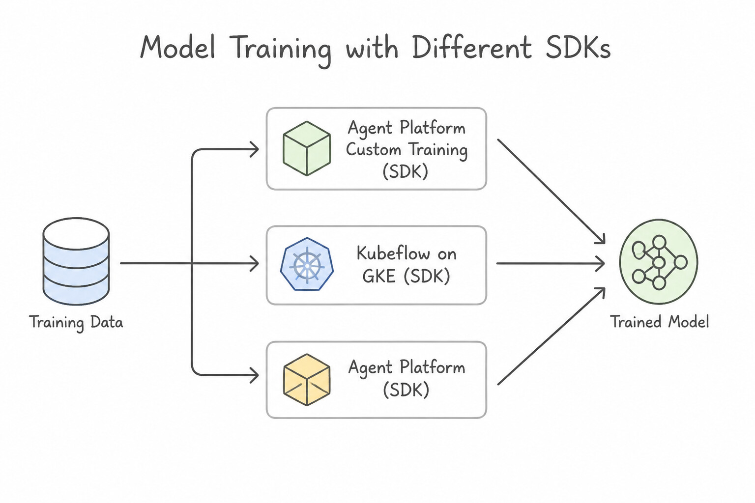
• Prebuilt Containers vs. Custom Containers in Agent Platform Custom Training:
• Use Prebuilt Training Containers (CustomTrainingJob / CustomJob with Python package distribution) when your TensorFlow, PyTorch, XGBoost, or Scikit-learn script only requires additional pure-Python PyPI packages (specified in setup.py or requirements.txt).
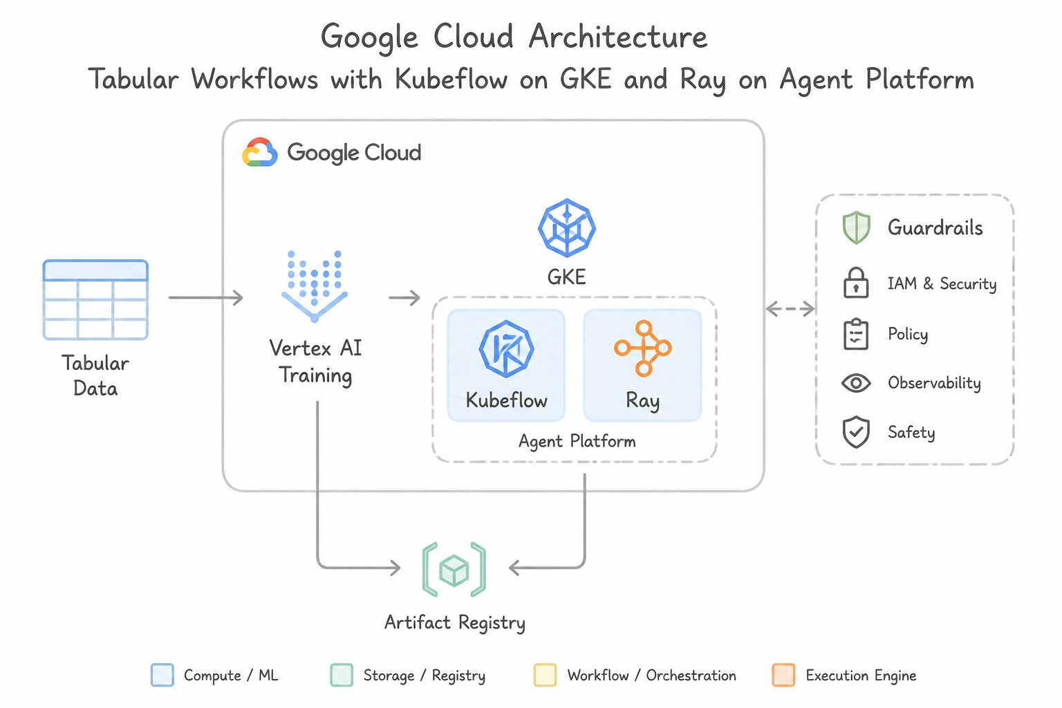
• Use Custom Training Containers when your code requires a non-supported framework version, custom OS-level binaries (apt-get), compiled C++ / Fortran libraries, or a custom entrypoint.
• Tabular Workflows, Kubeflow on GKE & Ray on Agent Platform:
• Tabular Workflows on Agent Platform: Provides managed, "glass-box" Kubeflow pipelines for AutoML Tabular where you can inspect intermediate artifacts, customize feature engineering steps, and scale to massive multi-terabyte datasets.
• Kubeflow on Google Kubernetes Engine (GKE): Choose when an organization requires strict hybrid-cloud portability (running the exact same Kubernetes/Kubeflow manifests on on-premises data centers and Google Cloud).
• Ray on Agent Platform: Choose when scaling distributed Python workloads, reinforcement learning, or fine-tuning jobs using the open-source Ray API (@ray.remote, Ray Train, Ray Tune) on managed Vertex AI clusters.

Key Implementation Patterns

• Custom Containers for Niche Dependencies: Use Create a custom container image that installs the C++ library and your code, then use this image for training. Custom containers allow you to install system-level dependencies required for your model training. (Avoid alternative: Requirements.txt only installs Python packages, not system-level C++ libraries.)
• Kubeflow on GKE for Hybrid Portability: Use Deploy Kubeflow on Google Kubernetes Engine (GKE) and use it for training. Kubeflow runs on Kubernetes, providing a consistent platform across on-premises clusters and GKE for seamless portability. (Avoid alternative: Vertex AI is a managed cloud service and does not run natively on standard on-premises Kubernetes clusters.)

Key Takeaways (3.2c)

• Use Pre-built Containers for standard frameworks and pure Python dependencies.
• Use Custom Containers when you need system-level libraries (C++, etc.) or specific OS configurations.
• Custom Containers are built using Docker and stored in Artifact Registry before being used in Vertex AI.
• Kubeflow is designed for portability across any Kubernetes environment (On-prem, GKE, AWS, Azure).

Consideration 3.2d: Troubleshooting ML model training failures

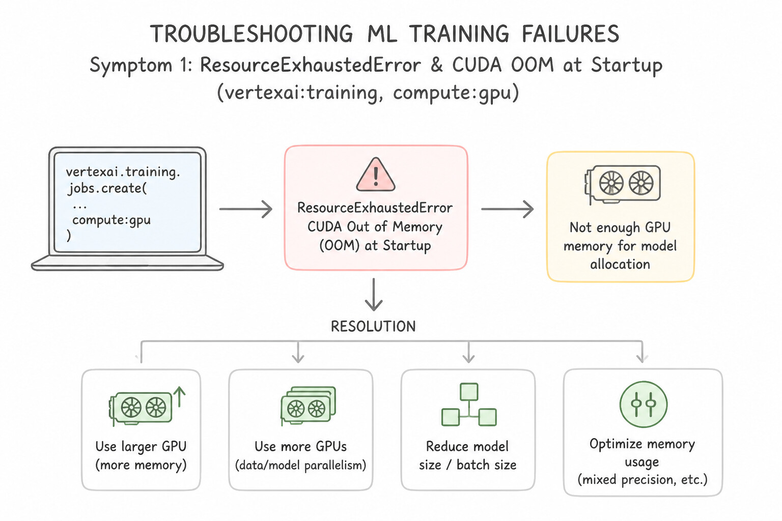
• Symptom 1 — ResourceExhaustedError / CUDA Out-of-Memory (OOM) at Startup:
• Root Cause: Batch activations + model weights + gradients + optimizer states exceed GPU VRAM.
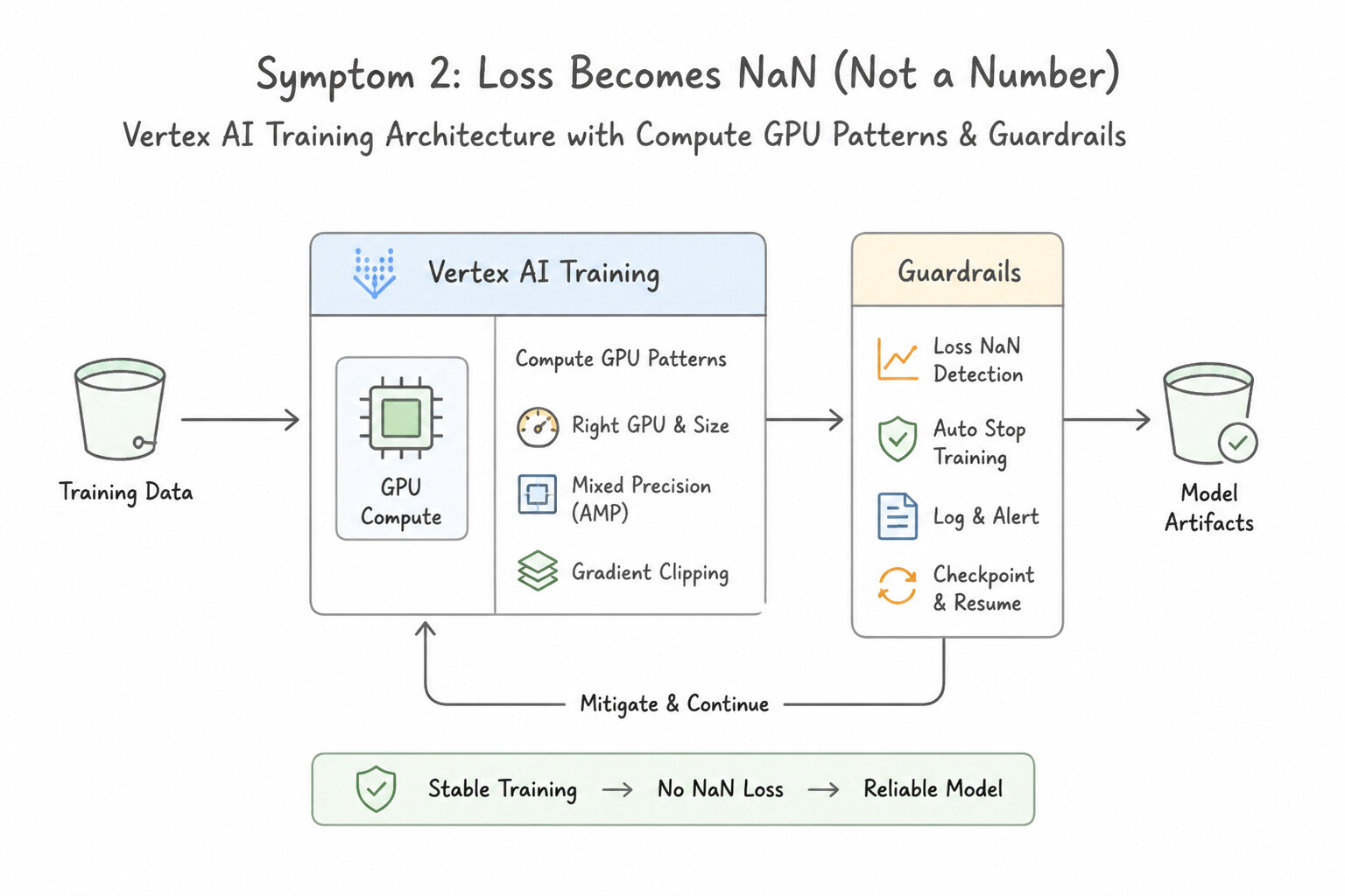
• Fixes: Reduce per-device batch size and enable Gradient Accumulation (accumulating gradients over $K$ micro-batches before calling optimizer.step(), preserving the large effective batch size without the memory spike), enable Mixed Precision (FP16 / bfloat16), or shard weights across devices via model parallelism / ZeRO.
• Symptom 2 — Loss Becomes NaN (Not a Number) During Training:
• Root Cause: Exploding gradients (common in RNNs and deep Transformers), an excessively high learning rate causing weight updates to overshoot into numerical overflow, log(0) operations, or corrupted NaN/Inf values in the input dataset.
• Fixes: Apply Gradient Clipping (clipnorm=1.0), lower the learning rate and add a Linear Warmup schedule, and validate inputs with TFDV / tf.debugging.check_numerics.
• Symptom 3 — GPU Utilization is <30% While CPU Utilization is 100%:
• Root Cause: Input I/O or CPU preprocessing starvation—the GPU finishes its forward/backward pass in milliseconds and sits idle waiting for the CPU to fetch and decode the next batch of small files from Cloud Storage.
• Fixes: Pack small files into TFRecords, add .prefetch(tf.data.AUTOTUNE) and parallel .map(), or offload preprocessing to Dataflow (tf.Transform).
• Symptom 4 — Distributed / Spot VM Job Preempted and Restarts from Epoch 0:
• Fix: Configure periodic checkpointing (ModelCheckpoint / tf.train.CheckpointManager) writing to the Cloud Storage URI exposed by the AIP_CHECKPOINT_DIR environment variable, and include startup logic to restore from the latest checkpoint if present.

Key Implementation Patterns

• Diagnosing Out of Memory (OOM) Errors on GPUs: Use Configure the training job to use a smaller batch size. OOM errors on GPUs are typically caused by a batch size that is too large; reducing the batch size lowers memory usage. (Avoid alternative: Adding more workers does not fix a per-device memory overflow if the local batch size remains too high.)
• Handling Gradient Explosion (NaN Loss): Use Configure the optimizer to use gradient clipping. Gradient clipping prevents exploding gradients by capping them at a maximum value. (Avoid alternative: Increasing the learning rate worsens gradient instability.)
• Synchronous Data Parallelism on a Single Machine: Use Instantiate a tf.distribute.MirroredStrategy object and build your model within the strategy's scope. MirroredStrategy is the standard TensorFlow API for synchronous training on a single machine with multiple GPUs. (Avoid alternative: MultiWorkerMirroredStrategy is intended for training across multiple different machines, not just a single machine with multiple GPUs.)

Key Takeaways (3.2d)

• ResourceExhaustedError (OOM) during GPU training usually means the Video RAM (VRAM) is full.
• The most common fix for OOM errors without changing hardware is to decrease the batch size.
• System RAM is separate from GPU VRAM; increasing system RAM does not fix GPU OOM errors.
• Scaling out (adding more workers) does not automatically fix per-device memory issues if the per-device batch size remains constant.

Consideration 3.2e: Hyperparameter tuning

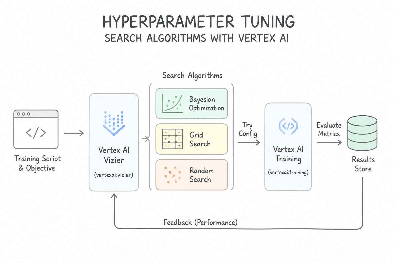
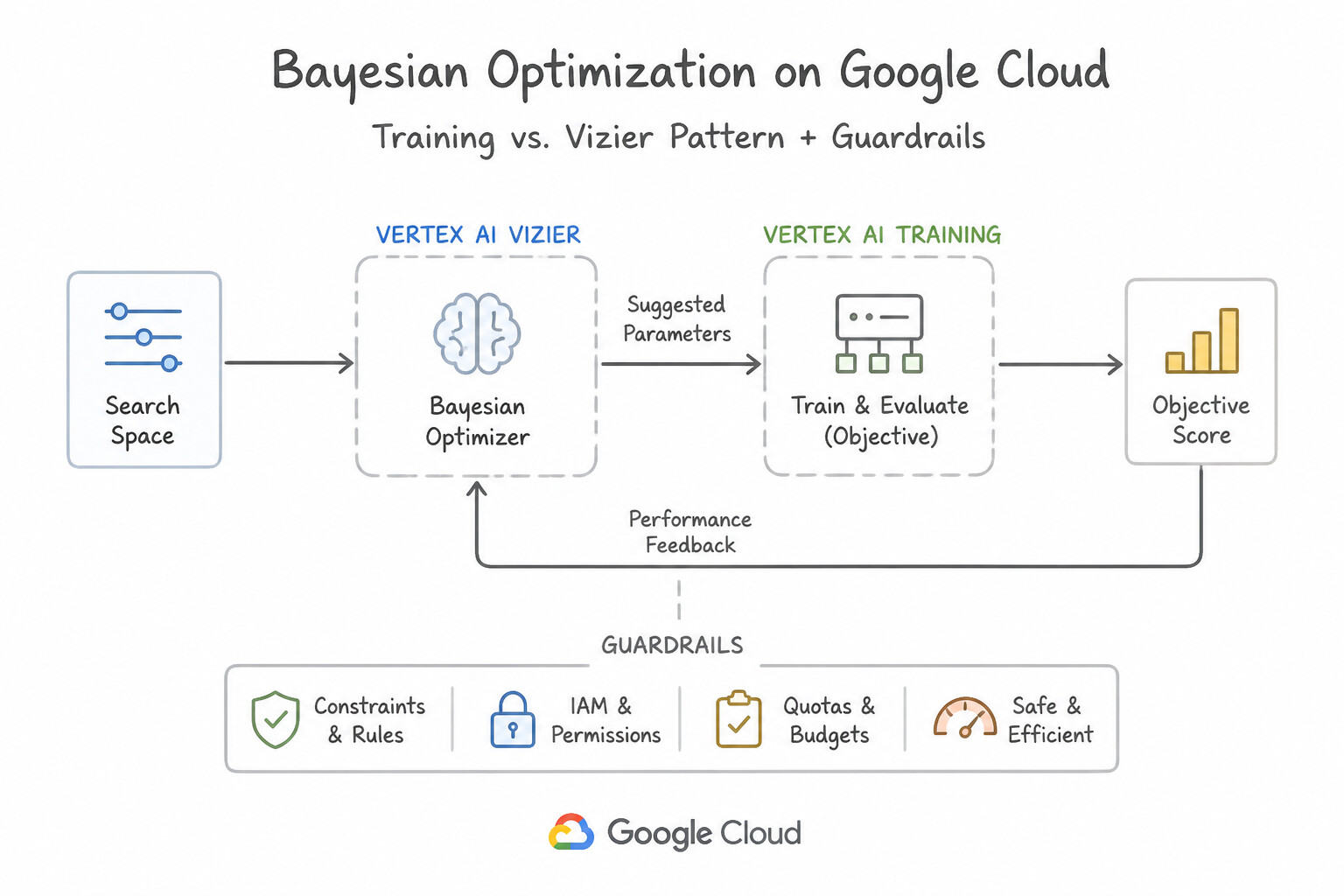
• Search Algorithms (Bayesian Optimization vs. Grid vs. Random):
• Bayesian Optimization (Default in Agent Platform / Vertex AI Vizier): Builds a Gaussian Process surrogate model of the objective function based on completed trials to intelligently select the next most promising hyperparameter configuration. Always choose Bayesian Optimization when training trials are expensive and the trial budget is limited.
• Grid Search only works for 1–2 discrete parameters; Random Search is useful when running massively parallel independent trials simultaneously.
• Parameter Scaling (UNIT_LOG_SCALE vs. UNIT_LINEAR_SCALE):
• When tuning parameters that span multiple orders of magnitude—such as learning_rate in [0.0001, 0.1] or regularization penalty \lambda in [1e-6, 1e-1]—always specify UNIT_LOG_SCALE. Using UNIT_LINEAR_SCALE on [0.0001, 0.1] wastes 90% of trials testing values between 0.01 and 0.1 while starving the critical 0.0001–0.001 region!
• Stopping Unpromising Trials Early (Median Automated Early Stopping): Enable Vizier's Median Automated Early Stopping (MedianStoppingConfig) (or DecayCurveAutomatedStoppingConfig) to automatically terminate any trial whose intermediate validation metric at step $t$ falls below the median of all completed trials at step $t$—slashing GPU compute costs.

Key Implementation Patterns

• Search Algorithm Efficiency: Use Configure Bayesian Optimization to select hyperparameter values based on the results of previous trials. Bayesian Optimization uses past trial data to intelligently choose the next parameters, minimizing the total trials needed. (Avoid alternative: Grid Search is too expensive and slow for large search spaces as it tests every combination.)
• Parameter Scaling Strategies: Use Set the scaling type to UNIT_LOG_SCALE. Logarithmic scaling explores orders of magnitude uniformly, which is necessary for parameters like learning rates. (Avoid alternative: Linear scaling biases the search toward larger numbers in the range, ignoring smaller orders of magnitude.)
• Cost Optimization with Stopping: Use Enable the automated early stopping feature in the study configuration. Automated early stopping automatically halts trials that perform poorly compared to completed trials, saving resources. (Avoid alternative: Reducing the number of trials limits the search scope and might prevent you from finding the best model.)

Key Takeaways (3.2e)

• Grid Search is systematic but expensive; use it only for very small search spaces.
• Random Search is better than Grid for high dimensions but is not 'smart'.
• Bayesian Optimization is the standard for modern ML tuning; it is iterative and efficient, making it ideal for limited budgets.
• Vertex AI Hyperparameter Tuning defaults to Bayesian Optimization (via Vizier) to maximize result quality with fewer trials.

Consideration 3.2f: Fine-tuning foundational models from Agent Platform and Model Garden and when tuning should be considered

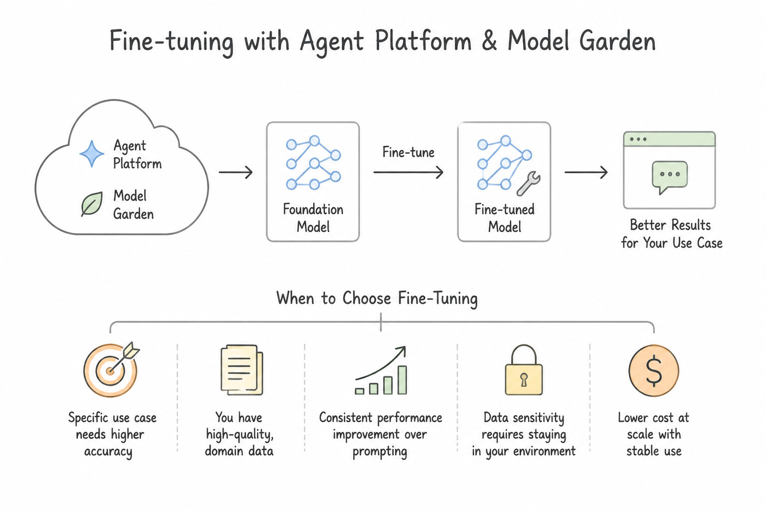
• When to Choose Fine-Tuning Over Prompting or RAG:
• Choose Supervised Fine-Tuning (SFT) when you need the model to internalize a specific output format, domain writing style, complex classification taxonomy, or specialized task behavior, or when you want to replace an expensive 50-example few-shot prompt with a zero-shot call to a smaller, faster tuned model (Gemini Flash).
• Do not use fine-tuning to inject rapidly changing daily facts (use RAG / Grounding instead).
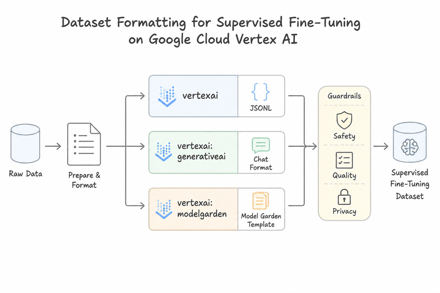
• Dataset Formatting for Supervised Fine-Tuning: Prepare a JSONL (JSON Lines) file in Cloud Storage where each line contains a structured training example: for classic text generation tuning, {"input_text": "...", "output_text": "..."} (or for Gemini chat/multimodal SFT, the contents / messages array with user and model roles).
• PEFT / LoRA vs. RLHF (Reinforcement Learning from Human Feedback):
• PEFT (LoRA / QLoRA): Freezes the base foundation model weights and trains lightweight low-rank adapter layers—drastically reducing GPU memory requirements, training cost, and the risk of catastrophic forgetting.
• RLHF: Choose when a fine-tuned model is factually accurate on domain tasks, but users report its conversational tone is robotic, overly terse, or misaligned with human helpfulness/safety preferences, and you have a dataset of human preference pairs (prompt, chosen_response, rejected_response) to train a Reward Model and align the policy.

Key Implementation Patterns

• Data Formatting for Supervised Fine-Tuning: Use Create a JSONL file where each line contains a JSON object with input_text and output_text fields. Vertex AI requires training data in JSONL format with specific input_text and output_text fields for text model tuning. (Avoid alternative: CSV is typically used for tabular data, not for fine-tuning generative text models on Vertex AI.)
• Reinforcement Learning from Human Feedback (RLHF): Use Tune the model using Reinforcement Learning from Human Feedback (RLHF). RLHF is the standard method for aligning models with human preferences using ranking data. (Avoid alternative: SFT uses examples to teach tasks, but it does not inherently leverage preference rankings for alignment.)
• Resolving Input Pipeline Bottlenecks (GPU Starvation): Use Use the tf.data API to implement prefetching and interleave the data loading process. High CPU and low GPU usage means the pipeline is input-bound; prefetching and parallel loading allow the CPU to feed the GPU faster.

Key Takeaways (3.2f)

• Vertex AI supervised fine-tuning for text models requires datasets in JSONL format.
• Each line in the training dataset must be a valid JSON object.
• The required keys for text generation models are input_text and output_text.
• Preparing clean, correctly formatted data is a critical first step in the ML workflow.

Quick Decision Cheat Sheet (Subsection 3.2)

Further Reading (Subsection 3.2)

• Best practices for Cloud Storage - Request rates and access distribution — Discusses performance considerations when using Cloud Storage, including the impact of small objects on throughput.
• Optimize the input pipeline - TensorFlow Core — Official TensorFlow documentation explaining the importance of using TFRecord and avoiding the overhead of reading small files.
• Read data from BigQuery with TensorFlow — This tutorial demonstrates how to use TensorFlow I/O to read data directly from BigQuery, leveraging the BigQuery Storage API for efficiency.
• BigQuery Storage API Overview — Provides details on the BigQuery Storage API, highlighting its ability to scan large datasets rapidly for consumers like machine learning models.
• Load data using Keras utility — Describes the standard directory structure expected by the image_dataset_from_directory utility, where images are organized into subdirectories representing their class.
• Prepare image data for Vertex AI — While Vertex AI AutoML often uses CSVs, custom training jobs on Vertex AI frequently rely on standard framework loaders that use the directory-based approach.

Subsection 3.3: Choosing appropriate hardware for training

Section 3: Scaling prototypes into ML models

The Big Picture

Choosing compute hardware and distributed training strategies on Google Cloud is where infrastructure engineering meets linear algebra. Provisioning the wrong accelerator or the wrong distribution strategy fails in four high-stakes ways:

1. Paying for GPUs/TPUs on CPU-Bound Classical Models—or Choosing TPUs for Custom CUDA / float64 Workloads (3.3a):
2. Standard Scikit-learn (and modest in-memory XGBoost) workloads run on CPU threads; attaching 8 NVIDIA A100 GPUs wastes thousands of dollars while the GPUs sit at 0% utilization.
3. Cloud TPUs are Google's custom ASICs with Matrix Multiply Units (MXUs) natively optimized for bfloat16 (BF16) and XLA-compiled static graphs (massive Transformers/CNNs in TensorFlow, JAX, or PyTorch/XLA). However, TPUs fail or degrade severely if your code relies on custom C++ CUDA kernels, strict float64 (double-precision) financial/scientific math, or heavy dynamic control flow / frequent host-CPU ops inside the training loop—those workloads belong on NVIDIA GPUs.
4. TPU Node vs. TPU VM Architecture (3.3a): Legacy TPU Nodes required a separate user Compute Engine VM communicating with a remote TPU host over gRPC—making interactive SSH debugging of NaN losses or host bottlenecks slow and opaque. Modern Cloud TPU VM architecture gives you direct SSH access onto the physical TPU host machine itself, eliminating network hop overhead and enabling direct local debugging.
5. Confusing Data Parallelism with Model Parallelism (3.3b):
6. Data Parallelism replicates the entire model onto every GPU/TPU core and shards the data batch across devices (MirroredStrategy for single-node multi-GPU, MultiWorkerMirroredStrategy for multi-node GPU, TPUStrategy for TPUs, PyTorch DistributedDataParallel [DDP]).
7. When a 500-billion-parameter LLM or a giant embedding table cannot fit into the HBM/VRAM of a single accelerator even at batch size 1, Data Parallelism crashes immediately with OOM! You must use Model Parallelism (Tensor/Pipeline Parallelism, FSDP, DeepSpeed ZeRO, or ParameterServerStrategy for huge embedding variables).
8. Network AllReduce Bottlenecks on Multi-Node GPU Clusters (3.3b): As synchronous data-parallel training scales from 2 GPU worker nodes to 32 GPU worker nodes, ring-AllReduce communication overhead across nodes grows until GPUs spend more time waiting on network gradient synchronization than computing. Enabling Vertex AI Reduction Server offloads and aggregates gradients across nodes using high-bandwidth tree/ring reductions, restoring near-linear scaling.

Consideration 3.3a: Evaluation of compute and accelerator options (e.g., CPU, GPU, and TPU)

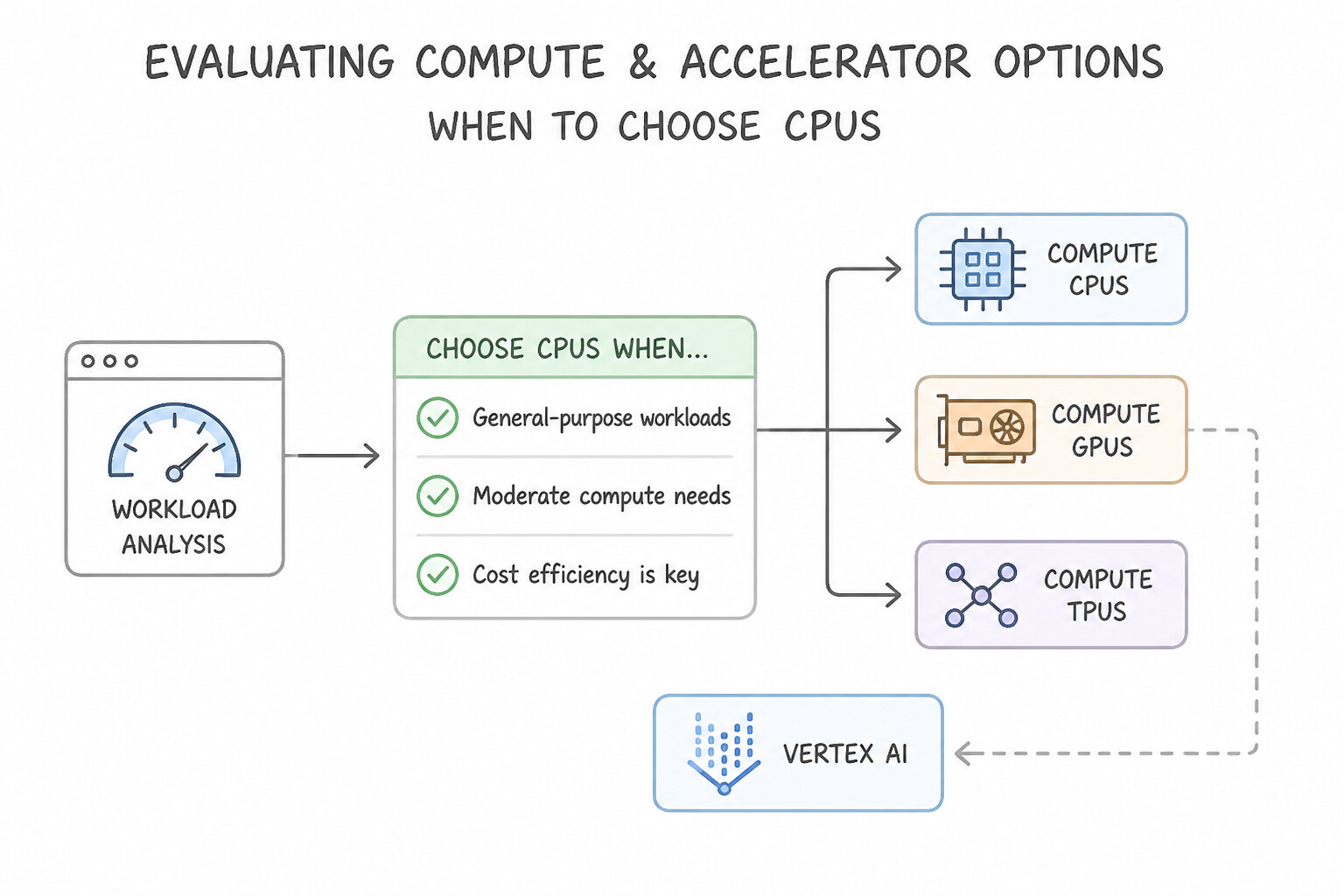
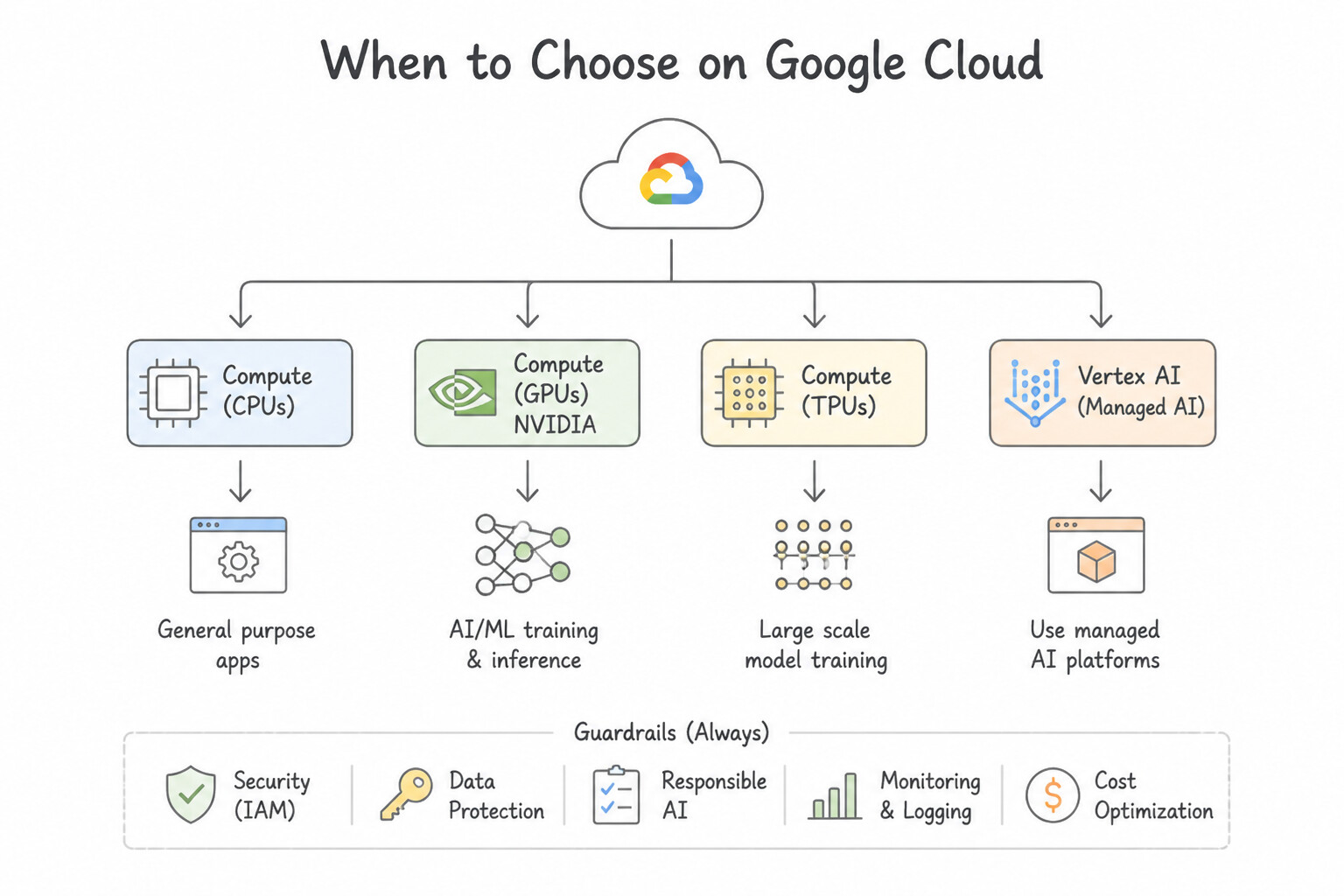
• When to Choose CPUs: Choose multi-core CPU VMs (e.g., n2-standard or n2-highmem) when training classical ML models (Scikit-learn, standard XGBoost, random forests, linear models) on tabular data that fits in memory. Adding GPUs or TPUs to a standard Scikit-learn job increases cost with zero speedup.
• When to Choose NVIDIA GPUs:
• Models written with custom C++ CUDA kernels or ops not supported by the XLA compiler.
• Quantitative finance or physics models requiring strict 64-bit floating-point (float64 / FP64) precision (TPUs natively operate in bfloat16/float32 and are unsuitable for strict float64 workloads).
• Workloads with heavy dynamic control flow, frequent CPU-GPU tensor transfers, or existing Horovod / PyTorch DDP multi-GPU containers.
• When to Choose Google Cloud TPUs (v4, v5e, v5p):
• Large-scale Transformers (LLMs) and CNNs dominated by dense matrix multiplications in TensorFlow, JAX, or PyTorch/XLA.
• Native bfloat16 (BF16) arithmetic: bfloat16 preserves the exact same 8-bit dynamic exponent range as float32 (preventing underflow/overflow without complex loss scaling) while using only 7 mantissa bits (16 bits total)—doubling memory bandwidth and MXU throughput.
• TPU VM vs. TPU Node: Always select TPU VM when you need direct SSH access to the TPU host for interactive debugging (e.g., attaching pdb, inspecting NaN tensors locally) and lower host-to-chip latency.
• TPU v4 / v5p Pod Interconnect: Uses Optical Circuit Switching (OCS) to dynamically route around failed racks and provide ultra-high-speed 3D torus all-reduce interconnects across thousands of chips.

Key Implementation Patterns

• Massive Scale LLM Training: Use Use Cloud TPU v4 Pods to distribute the training workload. TPU Pods are ASICs optimized for TensorFlow matrix operations and offer high-speed interconnects for cost-effective scaling of LLMs. (Avoid alternative: While powerful, GPUs are general-purpose accelerators; TPUs provide superior optimization and cost-efficiency specifically for large-scale TensorFlow workloads.)
• Custom Operations Constraint: Use Provision a machine type with NVIDIA GPUs for the training job. CUDA kernels are designed specifically for NVIDIA GPUs, making them the required hardware choice. (Avoid alternative: TPUs require XLA compatibility and do not natively support custom CUDA kernels.)
• Tabular Data Training: Use Provision a Compute Engine VM with a high-memory machine type and no accelerators. Scikit-learn and XGBoost generally rely on CPU instructions; a high-memory CPU instance is the most cost-effective choice for tabular data that fits in RAM. (Avoid alternative: Scikit-learn does not natively use GPUs, so paying for them adds cost without performance benefits.)

Key Takeaways (3.3a)

• TPUs are Google's custom ASICs optimized for TensorFlow and massive matrix operations.
• TPU Pods provide high-speed interconnects ideal for scaling large foundational models.
• GPUs are versatile but TPUs often offer better cost-efficiency for large-scale TensorFlow training.
• Edge TPUs and T4 GPUs are primarily for inference, not large-scale training.

Consideration 3.3b: Understanding the options for distributed training on GPUs and TPUs using data and model parallelism strategies

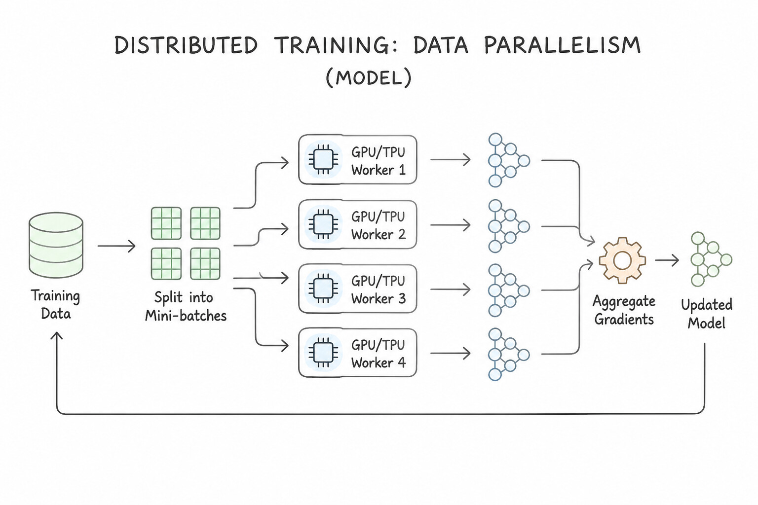
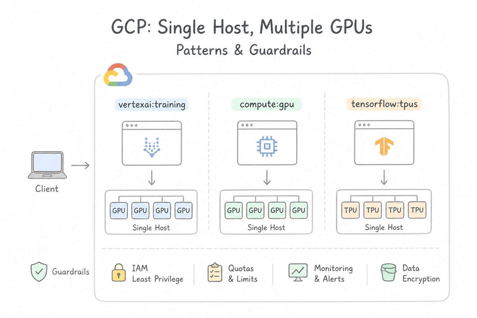
• Data Parallelism (Model Fits in Single Accelerator Memory): Every worker holds a complete replica of the model weights, processes a different shard of the mini-batch, and synchronizes gradients via AllReduce at the end of every step:
• Single Host, Multiple GPUs: tf.distribute.MirroredStrategy (uses NVIDIA NCCL over NVLink/PCIe).
• Multiple Hosts (VMs), Multiple GPUs: tf.distribute.MultiWorkerMirroredStrategy or PyTorch DistributedDataParallel (DDP) (configured with chief / workerPoolSpecs replica counts in Vertex AI).
• Cloud TPUs: tf.distribute.TPUStrategy (initialized after TPUClusterResolver.connect(), tf.config.experimental_connect_to_cluster, and tf.tpu.experimental.initialize_tpu_system, with model.compile() inside strategy.scope()).
• Accelerating Multi-Node GPU AllReduce with Vertex AI Reduction Server: When synchronous multi-node GPU training (MultiWorkerMirroredStrategy or Horovod) suffers from network bandwidth saturation as you scale worker nodes, add a Reduction Server pool in your Vertex AI custom job spec—it aggregates gradients using optimized topology-aware protocols and slashes inter-node communication time.
• Model Parallelism & Memory Sharding (Model Exceeds Single Accelerator Memory):
• When a 70B–500B parameter LLM or massive activation graph cannot fit on a single GPU/TPU even at batch size 1, you must partition the model itself:
• Tensor Parallelism (Intra-Layer) & Pipeline Parallelism (Inter-Layer): Splits individual weight matrices or sequential transformer layers across multiple accelerators in a TPU Pod slice or multi-GPU node.
• DeepSpeed ZeRO / PyTorch FSDP (Fully Sharded Data Parallel): Eliminates redundant memory copies across data-parallel ranks by sharding Optimizer States (ZeRO-1), Gradients (ZeRO-2), and Model Parameters (ZeRO-3 / FSDP) across all GPUs.
• Parameter Server Strategy (tf.distribute.ParameterServerStrategy): Asynchronous or sharded variable storage ideal when a recommendation model has a multi-hundred-gigabyte sparse embedding table that exceeds single-device memory.

Key Implementation Patterns

• Optimizing Gradient Updates with Vertex AI Reduction Server: Use Configure the training job to use Vertex AI Reduction Server. Vertex AI Reduction Server optimizes bandwidth and latency for the all-reduce gradient aggregation phase in distributed GPU training. (Avoid alternative: Adding more vCPUs increases compute power but does not resolve network bandwidth saturation between GPU nodes.)
• Migrating TensorFlow Code to TPUs: Use Initialize a TPUClusterResolver, create a tf.distribute.TPUStrategy, and wrap the model creation and compilation within strategy.scope(). TPUs require the tf.distribute.TPUStrategy and the model must be defined within strategy.scope().
• TPU Utilization and Code Scoping: Use Define the model architecture and compile the model inside a with strategy.scope(): block. The strategy.scope() context manager ensures variables and weights are created on the TPU devices. (Avoid alternative: Dataset creation usually happens on the CPU outside the strategy scope; the scope is for model variables.)

Key Takeaways (3.3b)

• Distributed training on multiple nodes requires synchronizing gradients (all-reduce).
• Network bandwidth often becomes a bottleneck as the number of GPU nodes increases.
• Vertex AI Reduction Server allows for optimized, high-throughput gradient aggregation for distributed GPU training.
• Reduction Server can be enabled without changing model architecture code.

Quick Decision Cheat Sheet (Subsection 3.3)

Further Reading (Subsection 3.3)

• Cloud TPU documentation — Provides an overview of Cloud TPU, explaining its architecture, benefits for TensorFlow workloads, and the concept of TPU Pods.
• TPU system architecture — Details how TPUs are interconnected and how they handle large-scale training jobs differently than standard GPU clusters.
• GPUs on Compute Engine — Documentation explaining that NVIDIA GPUs are available on Compute Engine and are used to accelerate CUDA-based workloads.
• Machine types | Compute Engine Documentation — Review the 'Memory-optimized machine types' section to understand when to use them for memory-intensive workloads.
• Optimize training performance with Reduction Server on Vertex AI | Google Cloud Blog — Explains how Reduction Server optimizes bandwidth and latency of the all-reduce collective operation for distributed training on Vertex AI.
• Use TPUs — The official TensorFlow guide on how to write code that runs on TPUs, including the use of TPUStrategy and scope.

Book TOC · Previous · Chapter 3 of 7 · Next