Book TOC · Previous · Chapter 3 of 6 · Next

Chapter 3: Enterprise Data Storage: BigQuery Warehousing, BigLake Lakehouses, Bigtable & Dataplex

Subsections Covered: 3.1, 3.2, 3.3, 3.4 (13 Considerations · 26 Custom Visual Diagrams)

Chapter Focus: Storage class lifecycles, BigQuery partitioning (ingestion/column) & clustering, nested/repeated STRUCT/ARRAY schemas, BigLake external tables (Apache Iceberg), Bigtable row-key design, and Dataplex governance.

Subsection 3.1: Selecting storage systems

Section 3: Storing the Data

The Big Picture

Section 3 (Storing the data, ~20% in Google Cloud architectures) opens with the foundational architectural decision of every data system: matching data access patterns to the right managed Google Cloud storage engine (3.1). Production architectures fail catastrophically when engineers force a database outside its physical design envelope:

1. The BigQuery-as-OLTP vs. Cloud SQL-as-Data-Warehouse Trap (3.1a, 3.1b): Using BigQuery to serve 20,000 point-lookup updates per second for a live shopping cart fails because BigQuery is a columnar OLAP engine with ~100ms+ query startup overhead and DML rate limits. Conversely, running petabyte-scale historical aggregations on a regional Cloud SQL instance saturates vCPUs and hits the 64 TB storage ceiling.
2. The Monotonic Key Hotspotting Disaster in Bigtable & Spanner (3.1a, 3.1c): Both Cloud Bigtable and Cloud Spanner split key ranges lexicographically across distributed storage tablets/splits. Starting a Bigtable row key with a raw timestamp (20261013190000#device123) or giving a Spanner table a SERIAL / auto-increment primary key routes 100% of writes to the single last node in the cluster, throttling a 50-node cluster down to 1-node throughput!
3. Storage Class Misalignment (3.1c, 3.1d): Leaving 2 PB of 5-year-old compliance logs in Cloud Storage Standard class wastes ratusan of thousands of dollars annually, whereas putting frequently read daily staging files into Archive class (365-day minimum duration + retrieval fees) triggers massive early-deletion penalties and read surcharges.

Consideration 3.1a: Analyzing data access patterns

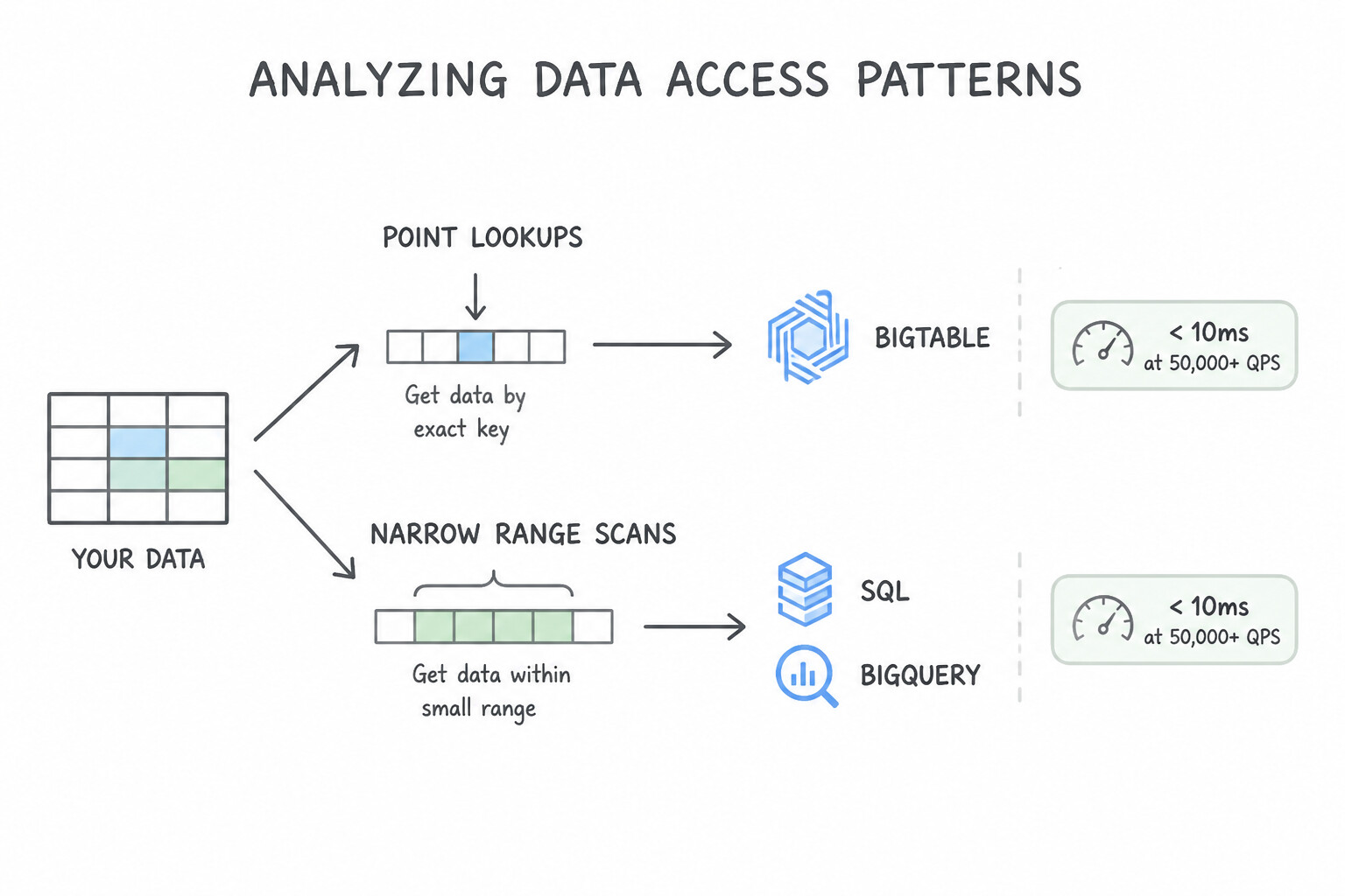
Translate scenario access-pattern keywords directly into architectural requirements:

• Point Lookups & Narrow Range Scans (< 10ms at 50,000+ QPS): Requires lexicographically indexed wide-column storage (Cloud Bigtable) where the exact fields queried in the WHERE clause form the Row Key prefix in order of cardinality/selectivity (tenant_id#device_id#reverse_timestamp).
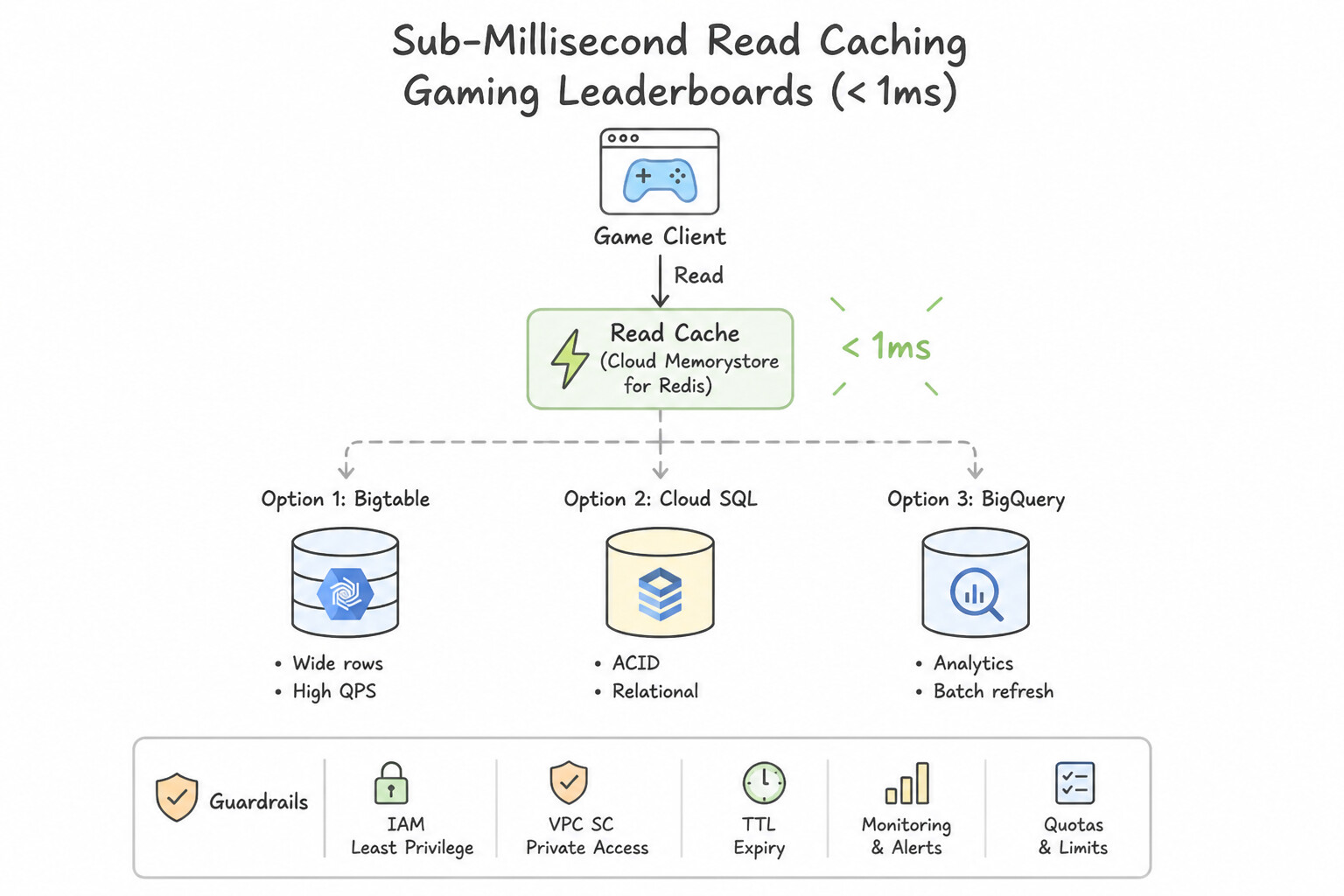
• Sub-Millisecond Read Caching & Gaming Leaderboards (< 1ms): Requires in-memory storage (Memorystore). Choose Memorystore for Redis when you need persistence (RDB/AOF), high-availability replica failover, Pub/Sub notifications, or advanced data structures (Sorted Sets ZADD/ZRANGE for leaderboards, Hashes, Lists). Choose Memorystore for Memcached only for simple, ephemeral, multi-threaded string key-value caching.
• Hybrid Transactional and Analytical Processing (HTAP): When a PostgreSQL application needs high-throughput OLTP writes and real-time analytical aggregations over the live operational tables without ETL delay, choose AlloyDB for PostgreSQL (which uses an automatic in-memory Columnar Engine).

Key Implementation Patterns

• High-Throughput IoT Ingestion: Use Use Bigtable to store the sensor data. Bigtable is designed for high-throughput, low-latency writes and handles time-series data efficiently. (Avoid alternative: Cloud SQL is a relational database not optimized for millions of concurrent writes per second.)
• Mobile Gaming User Profiles: Use Use Firestore to store the user profiles. Firestore is a NoSQL document store that natively supports offline synchronization and real-time updates for mobile apps. (Avoid alternative: Bigtable lacks native mobile SDKs for offline synchronization and real-time listeners.)
• Global Financial Transactions: Use Use Cloud Spanner with a multi-region configuration. Cloud Spanner provides the required global strong consistency, ANSI SQL support, and horizontal scaling for mission-critical financial applications. (Avoid alternative: Cloud SQL is regional and uses asynchronous replication for read replicas, which does not provide the strong global consistency needed for financial transactions.)

Key Takeaways (3.1a)

• Bigtable is the go-to service for high-throughput, low-latency writes (millions of writes/sec).
• IoT and time-series data are primary use cases for wide-column NoSQL stores.
• Relational databases (Cloud SQL) are better for transactional consistency, not raw ingestion speed.
• Object storage is for unstructured blobs, not high-frequency structured streams.

Consideration 3.1b: Choosing managed services (e.g., BigQuery, BigLake, AlloyDB, Bigtable, Spanner, Cloud SQL, Cloud Storage, Firestore, Memorystore)

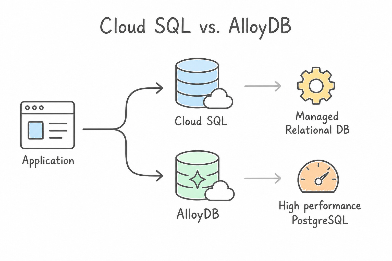
Memorize the exact boundaries between Google Cloud's 9 core storage services:

• Cloud SQL vs. AlloyDB vs. Cloud Spanner:
• Cloud SQL: Managed MySQL, PostgreSQL, or SQL Server up to 64 TB, vertical scaling (plus read replicas), regional HA (99.95% SLA). Best for lift-and-shift regional relational apps.
• AlloyDB for PostgreSQL: 100% PostgreSQL-compatible, up to 4x faster OLTP and 100x faster analytical queries (via its Columnar Engine) than standard PostgreSQL, 99.99% HA SLA (inclusive of maintenance), and built-in pgvector / Vertex AI integration.
• Cloud Spanner: Horizontally scalable relational database across regions/continents, External Consistency, 99.999% multi-region availability, unlimited scale. Best for global financial ledgers, global inventory, and multi-region ACID workloads.
• Firestore (Native Mode vs. Datastore Mode) vs. Cloud Bigtable:
• Firestore in Native Mode: Document-oriented NoSQL with real-time client listeners, mobile/web SDK offline persistence, and automatic scaling to zero.
• Firestore in Datastore Mode: Server-side high-throughput NoSQL for backend microservices compatible with legacy App Engine Datastore APIs.
• Cloud Bigtable: Wide-column HBase-compatible NoSQL for multi-terabyte to petabyte time-series, financial ticker, and IoT telemetry workloads.

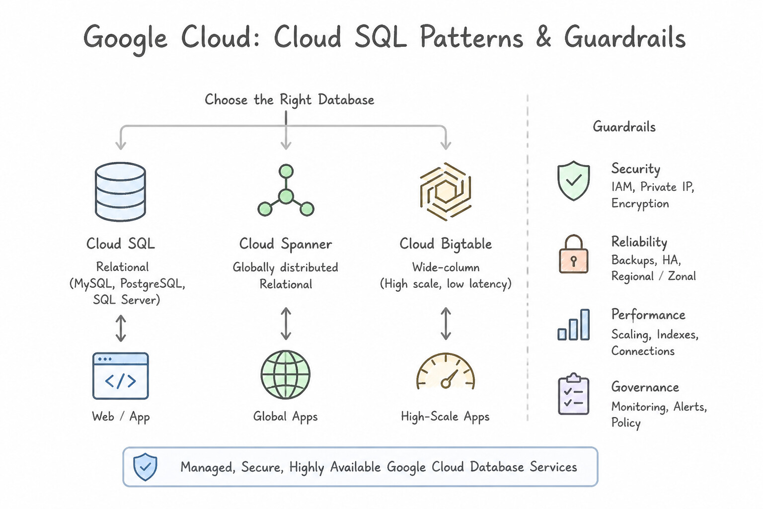
Key Implementation Patterns

• Global Transactional Consistency: Use Use Cloud Spanner configured with a multi-region instance configuration. Cloud Spanner provides global horizontal scaling, strong external consistency, SQL support, and 99.999% availability. (Avoid alternative: Cloud SQL is regional and does not support global horizontal write scaling or 99.999% availability.)
• High-Throughput IoT Ingestion: Use Store the data in Bigtable. Bigtable is optimized for high-throughput writes (millions/sec) and time-series data, making it the standard choice for IoT ingestion. (Avoid alternative: Firestore is designed for application development and document storage, not the massive write throughput required for high-volume IoT ingestion.)

Key Takeaways (3.1b)

• Cloud Spanner is the choice for global, horizontally scalable, relational (SQL) data.
• Cloud SQL is best for regional relational workloads up to a few terabytes.
• Strong external consistency combined with global scale is a defining feature of Spanner.
• 99.999% availability usually implies a multi-region Spanner configuration.

Consideration 3.1c: Planning for storage costs and performance

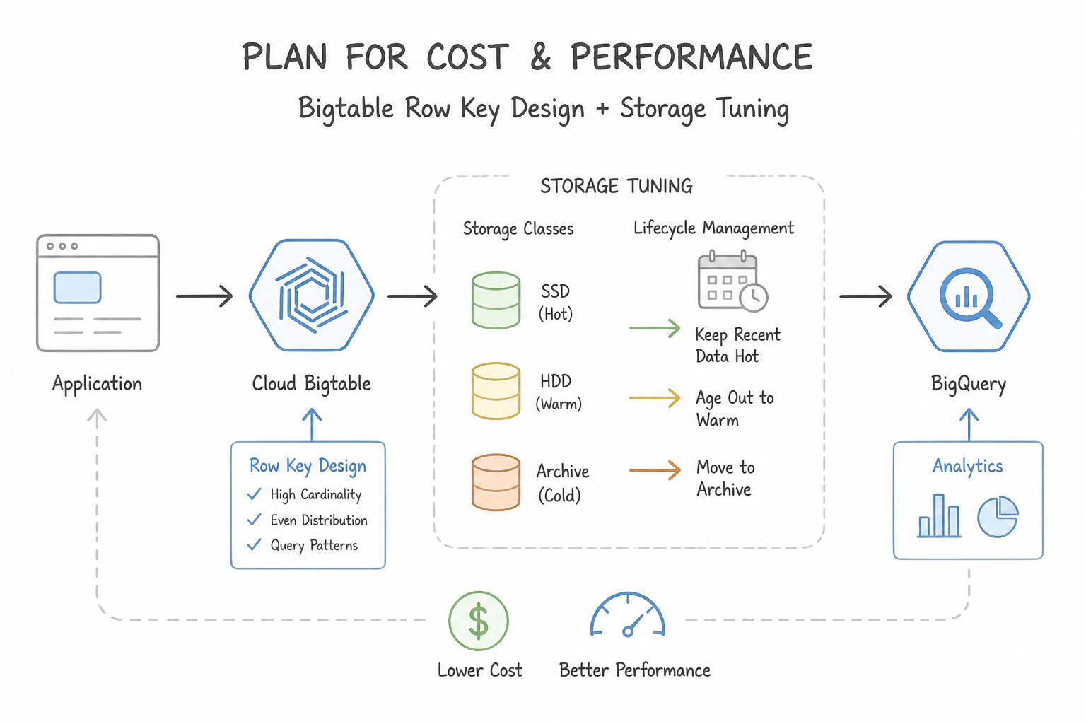
Master schema performance tuning and cost controls for Cloud Bigtable and Cloud Spanner:

• Cloud Bigtable Row Key Design & Storage Tuning:
• Avoid Hotspotting: Never start a row key with a timestamp, sequential ID, or low-cardinality boolean. Use Field Promotion / Salting / Compound Keys (sensor_type#location#device_id#(MAX_LONG - timestamp)). Using a reverse timestamp places the newest records at the top of the scan range so "get latest 100 readings for device_id" reads a single contiguous block!
• Tall and Narrow vs. Flat and Wide Tables: Prefer Tall and Narrow tables (one event per row, few columns) over adding thousands of timestamped columns to a single row (remember Bigtable's 100 MB cell / 256 MB row size limits).
• SSD vs. HDD Clusters: Always choose SSD (~10,000 read/write QPS per node, <10ms latency) for real-time serving and random reads. Choose HDD (~500 random read QPS per node!) only for large, cold, batch-scan-only archival workloads where random point lookups are never performed.
• App Profiles & Multi-Cluster Routing: Isolate batch Dataflow analytics from low-latency serving traffic by creating a Multi-Cluster Bigtable Instance; point real-time apps to Cluster A via a Single-Cluster Routing App Profile (or Multi-Cluster for HA read-only) and point batch jobs to Cluster B!
• Cloud Spanner Schema & Primary Key Design:
• Avoid Monotonic Primary Keys: Never use INT64 sequential counters or leading current-timestamp columns as the primary key in Spanner (causes split hotspotting). Use UUID v4, SHA-256 hash prefixes, bit-reversed sequences, or composite keys starting with a well-distributed shard ID.
• Interleaved Tables (INTERLEAVE IN PARENT): Physically co-locate child rows (OrderItems) with their parent row (Orders) in the same storage split to make parent-child joins ultra-fast single-split local reads.

Key Implementation Patterns

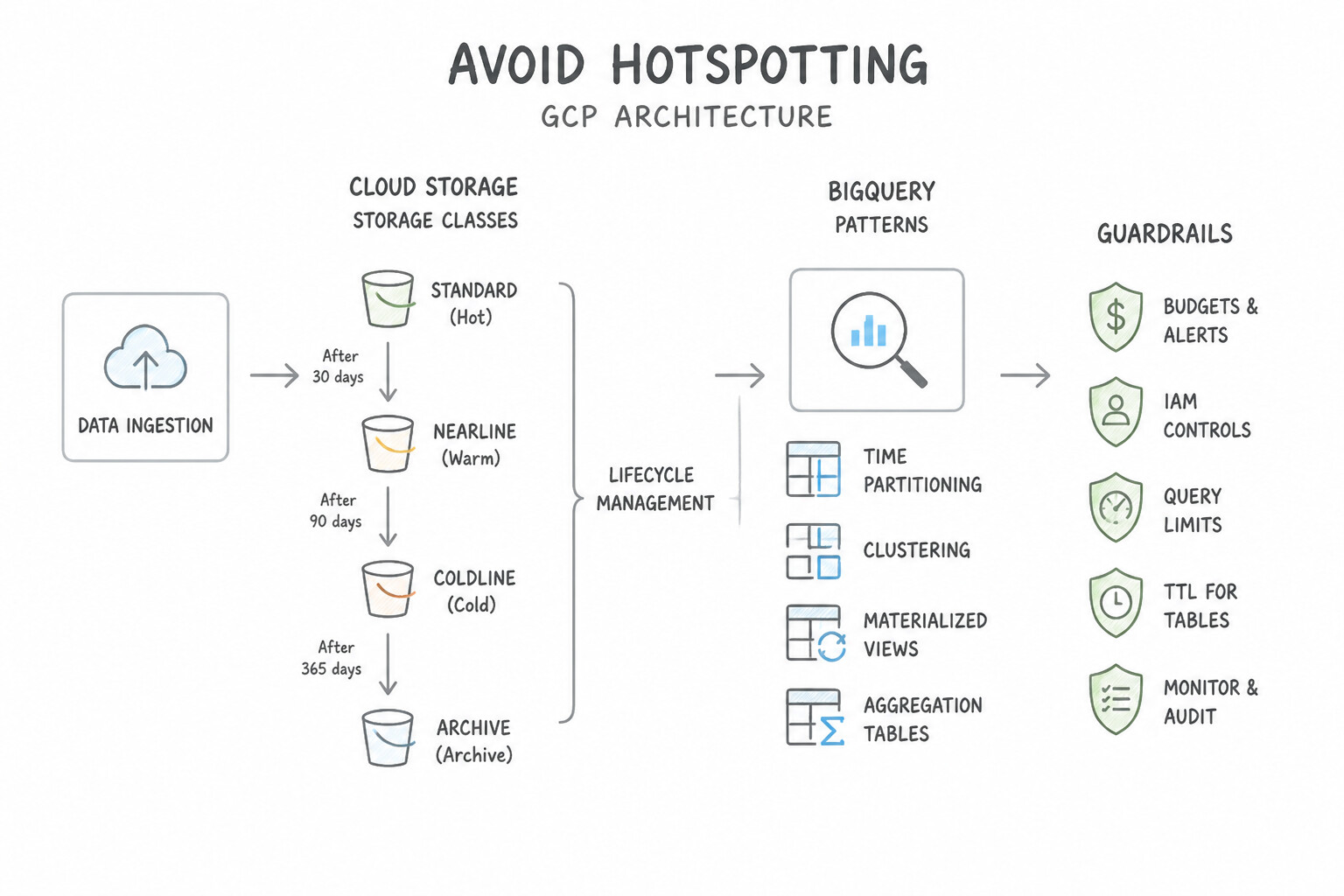
• Optimizing Cloud Storage for Regulatory Compliance: Use Create a Standard storage bucket. Configure an Object Lifecycle Management rule to change the storage class to Archive after 30 days. Standard storage handles the initial frequent access, and Archive storage offers the lowest cost for the remaining long-term retention.
• BigQuery Cost Optimization for Large Datasets: Use Partition the table by "transaction_date" and cluster by "customer_segment". Partitioning by date allows the query to skip irrelevant days, and clustering by segment organizes data to further minimize scanning. (Avoid alternative: Partitioning by segment does not optimize the primary date-based filter efficiently.)
• Bigtable Schema Design for Write Performance: Use Prepend a deterministic hash of the sensor ID to the row key. Hashing the sensor ID creates a random distribution of row keys, preventing writes from concentrating on a single node. (Avoid alternative: Timestamps at the start of a key cause all writes to hit the single node responsible for the current time range.)

Key Takeaways (3.1c)

• Match the storage class to the data access pattern (frequency).
• Use Standard for hot, active data.
• Use Archive for long-term retention and compliance data accessed less than once a year.
• Use Object Lifecycle Management to automate cost savings by moving aging data to colder storage classes.

Consideration 3.1d: Lifecycle management of data

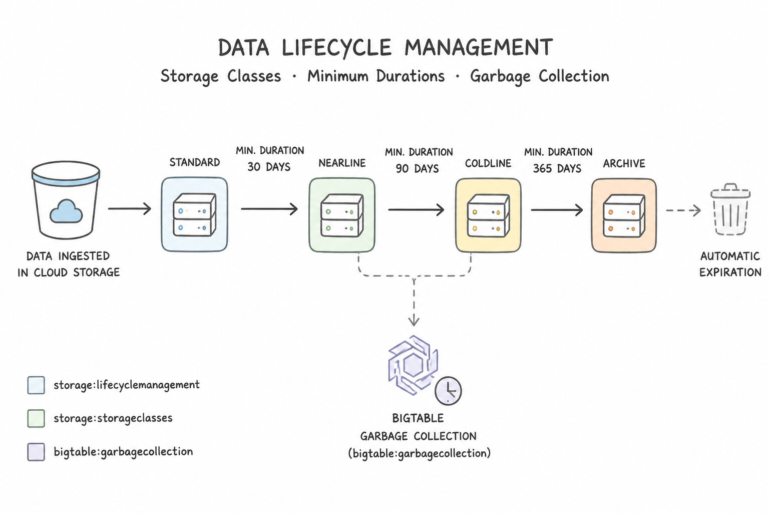
Automate data aging across Cloud Storage, BigQuery, and Cloud Bigtable so storage costs never grow unbounded:

• Cloud Storage Classes & Minimum Durations:
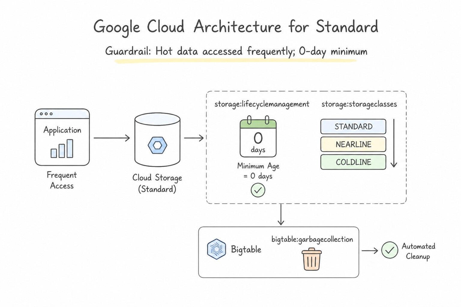
• Standard: Hot data accessed frequently; 0-day minimum storage duration, $0 retrieval fee.
• Nearline: Accessed ≤ 1 time per 30 days; 30-day minimum storage duration + per-GB retrieval fee.
• Coldline: Accessed ≤ 1 time per 90 days; 90-day minimum storage duration + higher per-GB retrieval fee.
• Archive: Accessed ≤ 1 time per 365 days; 365-day minimum storage duration + highest per-GB retrieval fee (note: millisecond first-byte latency, just like Standard!).
• Object Lifecycle Management (OLM) vs. Autoclass:
• Configure declarative Object Lifecycle Management rules (SetStorageClass to Nearline at Age: 30, Coldline at Age: 90, Archive at Age: 365, Delete at Age: 2555, plus DaysSinceNoncurrentTime for versioned buckets) when access patterns follow predictable calendar schedules.
• Enable Cloud Storage Autoclass when access patterns are unpredictable—Autoclass automatically transitions cold objects down to Nearline/Coldline/Archive and promotes them back to Standard upon read access without early-deletion penalties!
• Bigtable Garbage Collection (GC) & BigQuery Partition Expiration:
• In Cloud Bigtable, cell-level expiration is configured on the Column Family via Garbage Collection Policies (MaxAge e.g. 30 days, MaxVersions e.g. 1, combined via Union or Intersection). Note that Bigtable GC reclaims disk space asynchronously during compaction!
• In BigQuery, set default_partition_expiration_days on the table or dataset to automatically purge expired daily partitions at zero DML cost.

Key Implementation Patterns

• Cloud Storage Cost Optimization Rules: Use Create a rule to set the storage class to Nearline when the Age is 30 days. Create a second rule to set the storage class to Archive when the Age is 120 days. Combine the durations (30 + 90 = 120) to determine the Age for the second rule. Nearline is best for monthly access.
• Bigtable High-Volume Stream Cleanup: Use Configure a garbage collection policy using the union of max age 7 days and max versions 3. A Union policy keeps data if it matches either rule (Age OR Versions), satisfying both the recent history and latest value requirements. (Avoid alternative: Intersection requires data to meet both rules to stay, which would delete recent data that exceeds the version limit.)
• BigQuery Sandbox Cleanliness: Use Edit the dataset configuration and set the 'Default maximum table age' to 2 days. Setting the default table expiration at the dataset level ensures all new tables inherit this deletion policy automatically. (Avoid alternative: Manual processes are unreliable and do not strictly enforce the automatic deletion requirement.)

Key Takeaways (3.1d)

• Age Calculation: Lifecycle 'Age' is always calculated from the object's creation date, not the date of the previous transition.
• Class Selection: Match storage classes to access frequency: Nearline (monthly), Coldline (quarterly), Archive (yearly).
• Cost Optimization: Use Lifecycle Management to automate tiering and reduce storage costs without manual intervention.
• Garbage Collection is defined at the Column Family level.

Quick Decision Cheat Sheet (Subsection 3.1)

Further Reading (Subsection 3.1)

• Cloud Bigtable Overview — Read the section on 'What is Cloud Bigtable?' to understand its design for high throughput and scalability.
• Time series data schema design — This page specifically discusses why Bigtable is suitable for time-series data and how to structure keys.
• Firestore features — Overview of Firestore capabilities including flexible data model, offline support, and real-time updates.
• Enable offline data — Documentation explaining how Firestore allows you to access data offline and syncs changes when back online.
• Cloud Spanner Overview — Provides an introduction to Cloud Spanner, highlighting its global scale, strong consistency, and SQL support.
• Cloud Spanner vs. Cloud SQL — A guide helping to choose between Google Cloud database options based on requirements like global scale and consistency.

Subsection 3.2: Planning for using a data warehouse

Section 3: Storing the Data

The Big Picture

Engineers migrating from legacy row-oriented databases (Oracle, SQL Server, Teradata) often bring 3rd Normal Form (3NF) habits into BigQuery—splitting a single Order across 8 normalized tables (orders, order_items, customers, addresses, promotions) and joining them at query time across 50 TB of data. In BigQuery's distributed Capacitor columnar storage and Borg shuffle architecture, that design wastes massive slot capacity:

1. The Distributed Shuffle JOIN Tax vs. Nested & Repeated ARRAY<STRUCT> (3.2a, 3.2b): In BigQuery, storage is cheap while distributed network shuffles (JOIN across large tables) consume the bulk of slot time. When a 1-to-many relationship is queried together 90% of the time (such as an Order and its LineItems), denormalizing the child records into a Nested and Repeated column (ARRAY<STRUCT<...>> / RECORD REPEATED) co-locates parent and child data inside the same physical Capacitor file block—turning an expensive distributed shuffle JOIN into a zero-network-hop local UNNEST() operation!
2. The 4,000-Partition Ceiling & Full-Table Scan Trap (3.2d): BigQuery allows a maximum of 4,000 partitions per table. If an enterprise must retain 15 years of historical IoT or financial data (15 × 365 = 5,475 days), daily partitioning fails! The winning architecture uses Monthly (or Yearly) partitioning combined with Clustering on the timestamp/entity columns, plus require_partition_filter = true.
3. Expensive Table Copies for Backup & Testing (3.2c, 3.2d): Copying a 100 TB production table (CREATE TABLE AS SELECT) for before-upgrade backups or developer sandbox testing doubles storage costs immediately. BigQuery provides 7-day Time Travel (FOR SYSTEM_TIME AS OF), Table Snapshots (immutable point-in-time backups that charge only for changed delta bytes), and Table Clones (writable zero-copy sandboxes that charge only for modified blocks).

Consideration 3.2a: Designing the data model

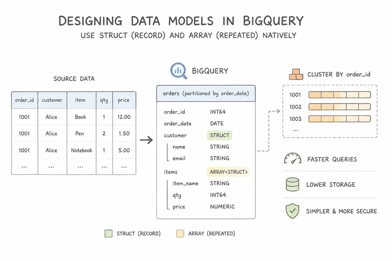
Design schemas specifically for BigQuery's Capacitor columnar storage format:

• Use STRUCT (Record) and ARRAY (Repeated) Natively:
• A STRUCT groups related attributes (e.g., shipping_address.city, shipping_address.zip) under a single namespace; Capacitor still stores each sub-field as an independent physical column, so querying SELECT shipping_address.zip scans only the zip sub-column!
• An ARRAY<STRUCT<...>> (REPEATED RECORD) stores multiple child rows (e.g., line_items inside an order, or events inside a session) inline within a single parent row.
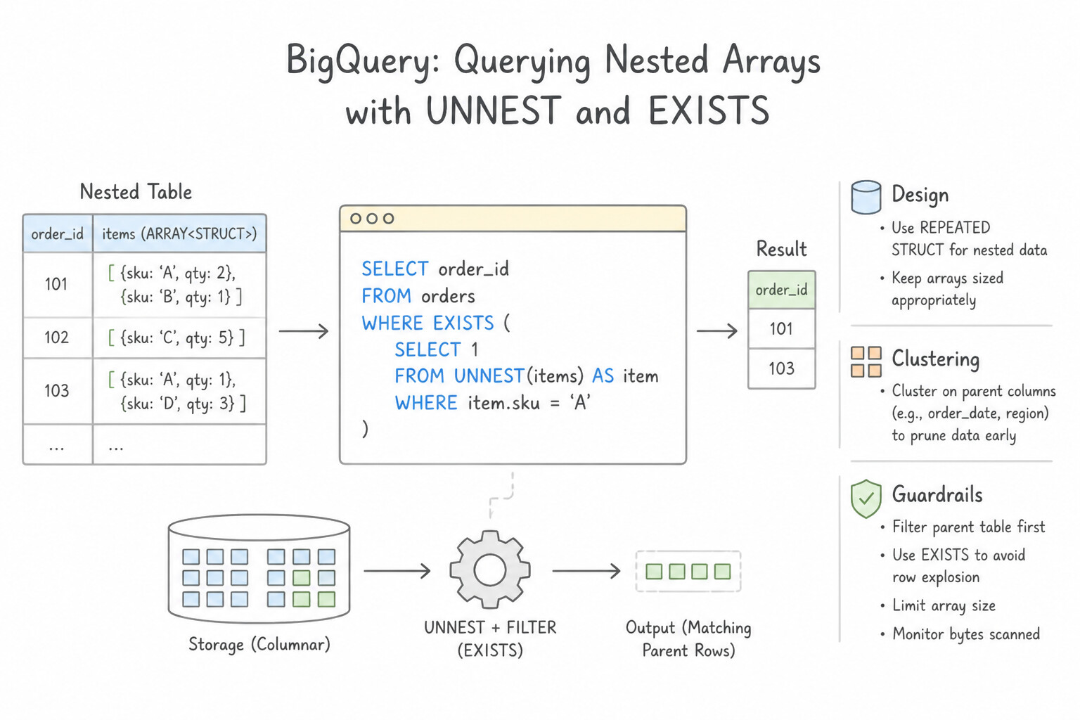
• Querying Nested Arrays with UNNEST and EXISTS:
• Use CROSS JOIN UNNEST(line_items) AS item (or comma-join , UNNEST(line_items)) only when you need to flatten the array into one output row per array element.
• To filter parent rows based on an array condition without multiplying parent rows, use a correlated subquery: WHERE EXISTS (SELECT 1 FROM UNNEST(line_items) AS item WHERE item.category = 'Electronics').

Key Implementation Patterns

• Denormalization with Nested and Repeated Fields: Use Denormalize the schema by creating a single table with one row per order and nesting "Order_Items" as an ARRAY of STRUCTs. Using nested and repeated fields eliminates joins and optimizes read performance in BigQuery. (Avoid alternative: Views do not store data physically and will still execute the underlying join operation at runtime.)
• Clustering for High Cardinality Filtering: Use Update the table definition to cluster by customer_id and region. Clustering organizes data within partitions, allowing BigQuery to skip scanning irrelevant data blocks when filtering by high-cardinality columns. (Avoid alternative: Partitioning is limited to 4,000 partitions and is not suitable for high-cardinality columns like unique customer IDs.)
• Partitioning Strategy for Time-Series Data: Use Create a new table partitioned by the log timestamp. Migrate the data to the new table. Partitioning by timestamp allows queries to scan only the specific days requested, drastically reducing costs. (Avoid alternative: BigQuery does not use traditional secondary indexes to reduce scan costs for date ranges; partitioning is the correct tool.)

Key Takeaways (3.2a)

• Joins in distributed systems are expensive; avoid them when possible for high-volume queries.
• BigQuery supports nested and repeated fields (ARRAY of STRUCTs) to handle one-to-many relationships efficiently.
• Denormalization improves read performance at the cost of slightly more complex data loading logic.
• Partition tables by date or timestamp to manage data lifecycle and reduce scan costs for time-based queries.

Consideration 3.2b: Deciding the degree of data normalization

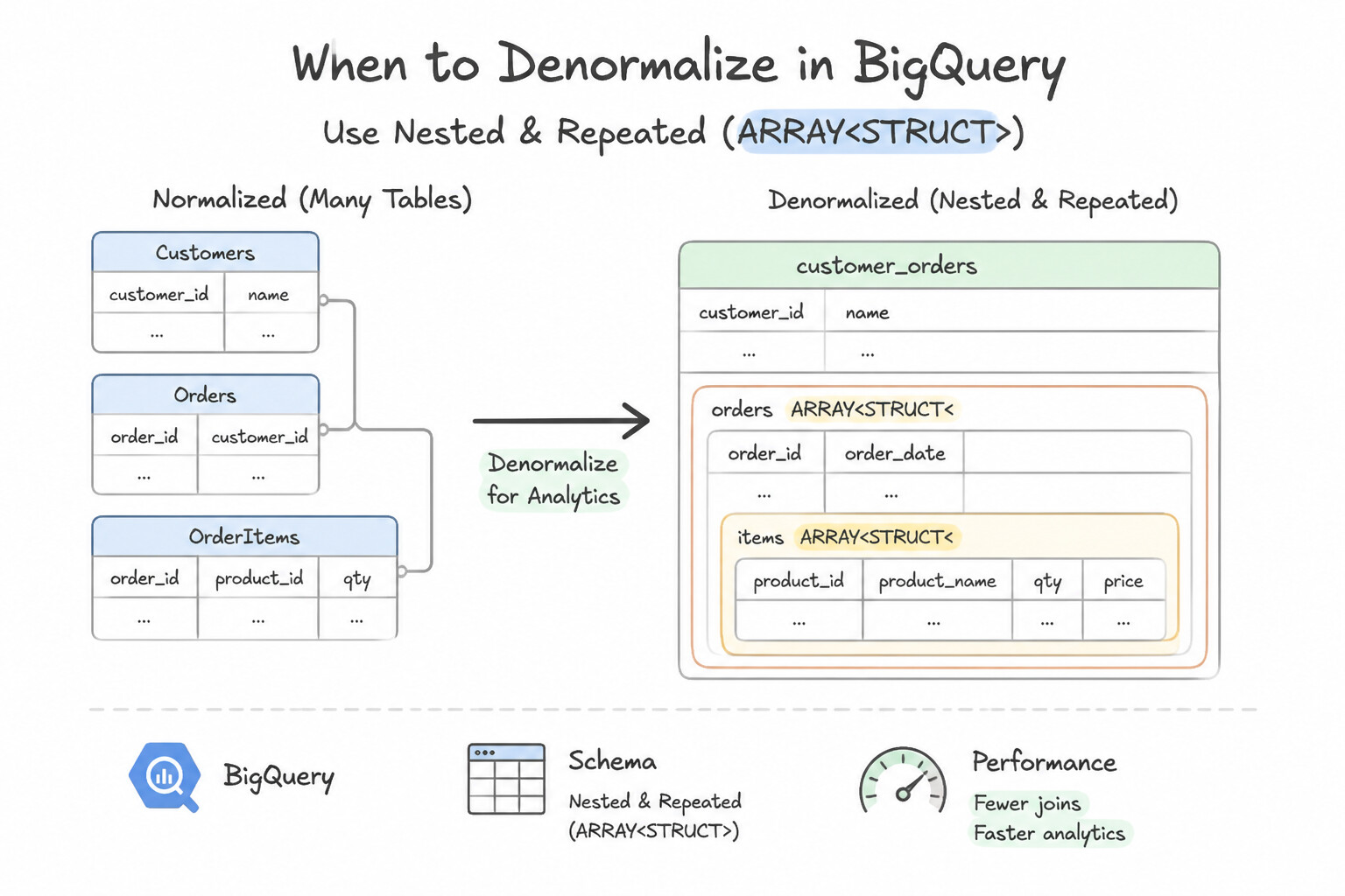
In Google Cloud architectures, "always denormalize everything into one giant flat table" is a trap when dimension attributes change frequently! Apply this exact rule:

• When to Denormalize (Nested & Repeated ARRAY<STRUCT>):
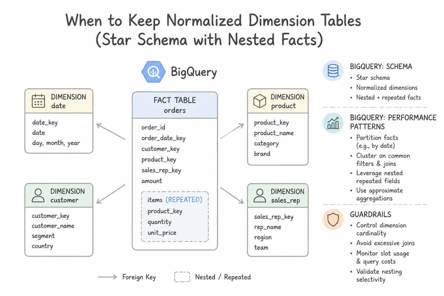
• Immutable or append-only 1-to-many transactional facts (e.g., Orders + Order_Line_Items, Web_Sessions + Page_Views, Invoices + Charges). Denormalizing into ARRAY<STRUCT> eliminates shuffle joins and reduces storage footprint (because parent columns are not repeated across every child row as they would be in a flat wide table!).
• When to Keep Normalized Dimension Tables (Star Schema with Nested Facts):
• When a dimension table (e.g., Customers or Products with 50 attributes) experiences frequent UPDATE / DELETE mutations (e.g., customer changes address or loyalty tier daily). If you hardcoded those 50 customer attributes into a 200 TB Sales_Fact table, updating a customer's tier would require rewriting terabytes of historical fact partitions via expensive DML! Instead, store customer_id on the nested Sales_Fact table and join the small Customers dimension table (which BigQuery optimizes via Broadcast Join).

Key Implementation Patterns

• Optimizing Read Performance with Nested Fields: Use Denormalize the schema by using nested and repeated fields for Product data within the Sales table. Denormalization using nested fields eliminates the need for expensive joins, resolving the latency caused by shuffling.
• One-to-Many Relationships (Arrays): Use Create a table with a REPEATED RECORD column to store the array of readings within a single row per batch. Using REPEATED fields allows you to nest multiple readings in a single row, optimizing performance and storage. (Avoid alternative: Storing one row per reading multiplies the row count significantly, which is inefficient for BigQuery performance and storage.)
• Handling Frequent Dimension Updates: Use Design a normalized schema. Store Login Logs and User Profile in separate tables and join them on a user ID. Normalize the schema to handle frequent dimension updates efficiently without rewriting historical fact data. (Avoid alternative: Nested fields do not solve the update churn problem for shared mutable dimensions.)

Key Takeaways (3.2b)

• Joins between large tables cause data shuffling, which increases query latency in distributed systems.
• BigQuery performs best with denormalized data schemas.
• Use nested (STRUCT) and repeated (ARRAY) fields to locate related data together and avoid expensive joins.
• Do not apply OLTP normalization rules (like 3NF) blindly to OLAP warehouses like BigQuery.

Consideration 3.2c: Mapping business requirements

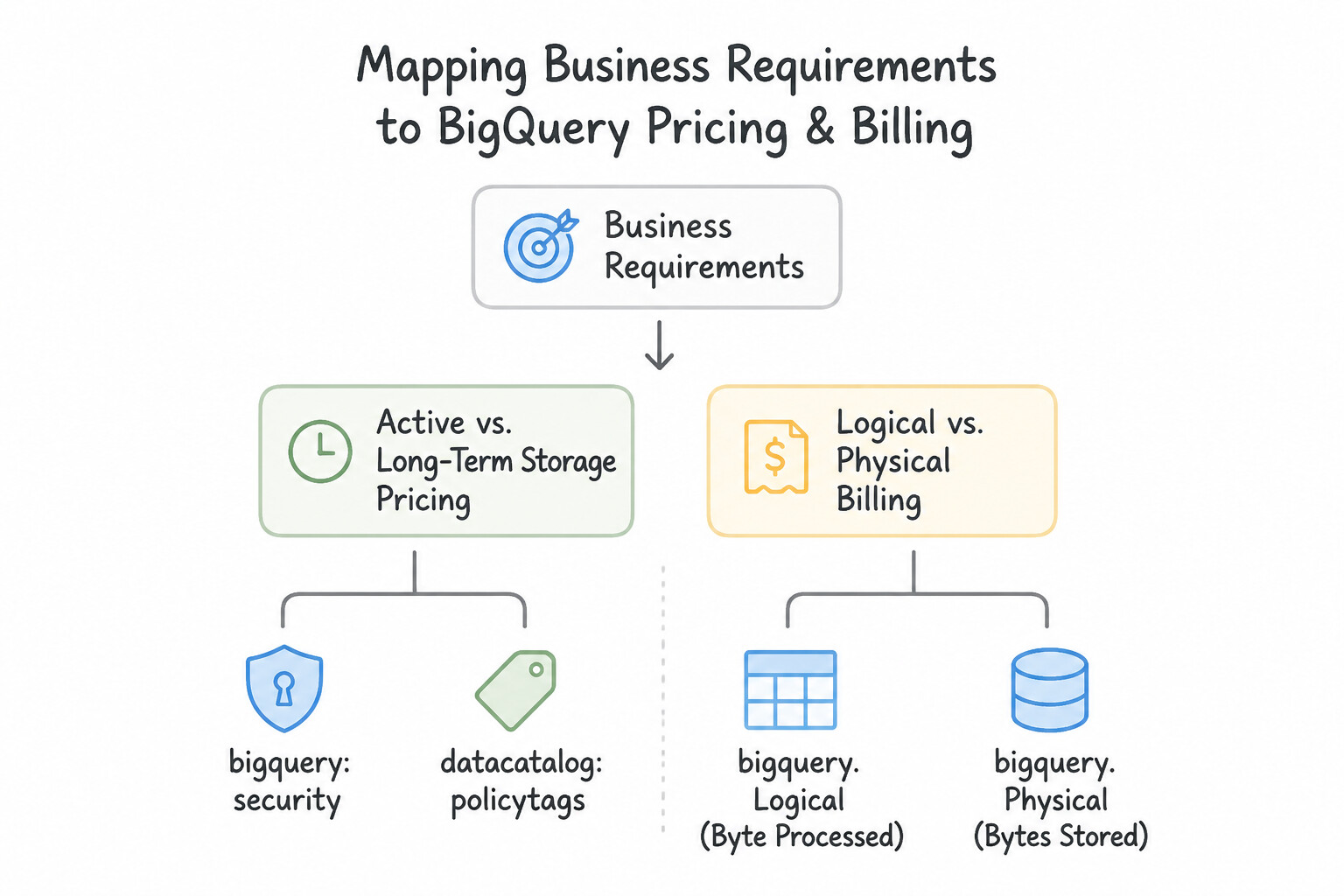
Master BigQuery's storage economics and zero-copy table primitives:

• Active vs. Long-Term Storage Pricing & Logical vs. Physical Billing:
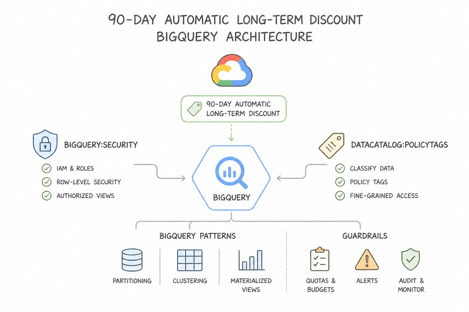
• 90-Day Automatic Long-Term Discount: Any table or partition that is not modified (INSERT, UPDATE, DELETE, LOAD, COPY) for 90 consecutive days automatically drops in storage price by ~50% (Active → Long-Term). Architecture Tip: Reading (SELECT) a table or changing its IAM/description metadata does not reset the 90-day timer!
• Physical (Compressed) vs. Logical (Uncompressed) Storage Billing: Datasets can be configured to bill by Physical (Compressed) bytes (including Time Travel + 7-day Fail-safe bytes) rather than Logical uncompressed bytes—often saving 40–70% on highly compressible text/repetitive datasets that have low DML churn.
• Time Travel vs. Table Snapshots vs. Table Clones:
• Time Travel (FOR SYSTEM_TIME AS OF): Built-in window (configurable 2 to 7 days, default 7 days) to query or restore a table as it existed at any millisecond in the past. (Followed by a 7-day Google-support-only Fail-safe period).
• Table Snapshots (CREATE SNAPSHOT TABLE): Lightweight, read-only point-in-time backups that persist beyond 7 days (for months or years). Initial storage cost is $0; you pay only for bytes deleted or modified in the base table after the snapshot was taken.
• Table Clones (CREATE TABLE ... CLONE source_table): Lightweight, read/write (mutable) independent copy of a table created in seconds. Initial storage cost is $0; you pay only for new/modified data blocks written to the clone. Ideal for developer testing sandboxes!

Key Implementation Patterns

• Strict PII Access Control: Use Create Data Catalog policy tags for sensitive columns and grant the Data Catalog Fine-Grained Reader role to the auditors. Policy tags enable column-level security, allowing granular access control on specific fields without managing multiple views.
• High-Performance Read Optimization: Use Consolidate the data into a single table using nested and repeated fields for the order items. Nested and repeated fields allow you to store parent-child relationships in a single table, eliminating slow joins. (Avoid alternative: Normalized schemas require joins, which are slower and more resource-intensive in BigQuery.)

Key Takeaways (3.2c)

• Use BigQuery Column-Level Security to restrict access to specific fields (columns) containing sensitive data.
• Policy Tags (via Data Catalog/Dataplex) are the mechanism for defining and enforcing these column restrictions.
• Avoid creating multiple Authorized Views for simple column hiding if a native security feature (Policy Tags) can achieve the same result with less management overhead.
• Row-Level Security filters rows; Column-Level Security filters columns.

Consideration 3.2d: Defining architecture to support data access patterns

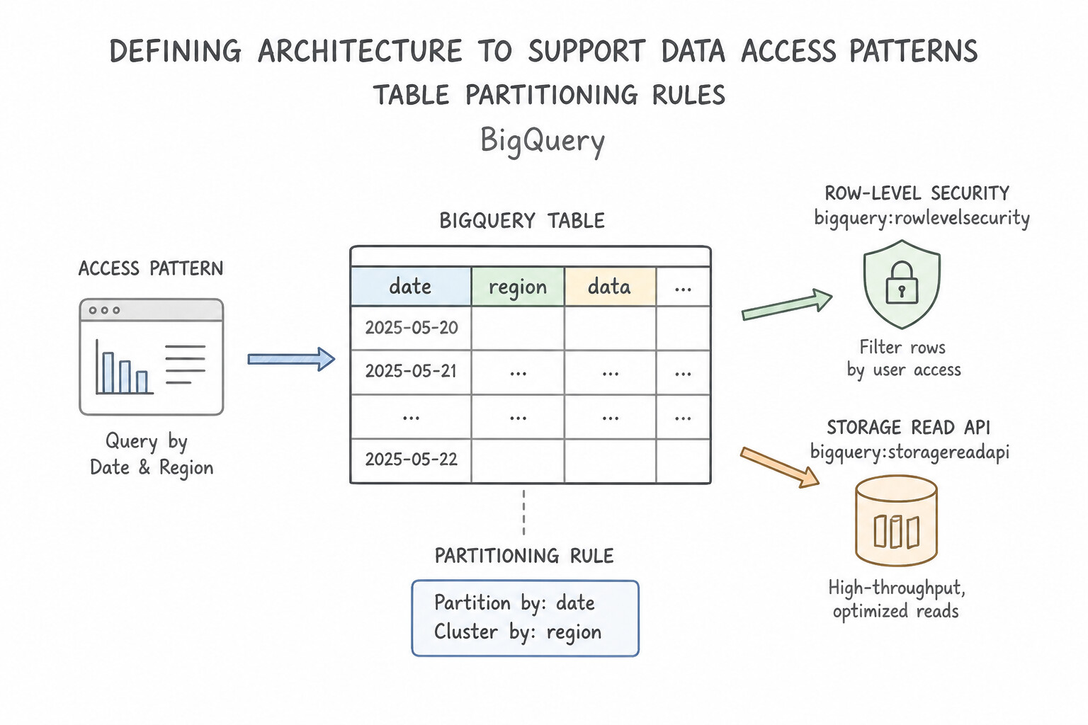
Always combine Partitioning and Clustering properly:

• Table Partitioning Rules:
• Types:
• Time-Unit Column (DATE, TIMESTAMP, DATETIME): Granularity can be Hourly, Daily (default), Monthly, or Yearly.
• Ingestion-Time (_PARTITIONTIME / _PARTITIONDATE): Automatic partitioning when source records lack a reliable event timestamp.
• Integer-Range (RANGE_BUCKET(customer_id, GENERATE_ARRAY(0, 100000, 100))): Partitioning on an integer ID column.
• The 4,000-Partition Hard Limit: A single BigQuery table can have at most 4,000 partitions. For 15 years of data (5,475 days) or 5 years of hourly data (43,800 hours), daily/hourly partitioning fails—choose Monthly Partitioning + Clustering on the event_timestamp column!
• Cost Guard (require_partition_filter = TRUE): Forces every SELECT query to include a constant filter on the partitioning column, preventing accidental full-table scans.
• Partition Pruning Trap: Wrapping the partition column in a function (WHERE EXTRACT(YEAR FROM order_date) = 2026 or WHERE DATE(event_ts) = CURRENT_DATE()) or comparing against a dynamic subquery defeats partition pruning in many cases—always filter directly on the partition column against literal/parameter bounds (WHERE event_ts >= '2026-01-01' AND event_ts < '2026-02-01').
• Table Clustering Rules:
• Specify up to 4 columns (CLUSTER BY col1, col2, col3, col4).
• Column Order Is Critical: Place the most frequently filtered or aggregated high-cardinality column first (col1), followed by the second most frequent (col2), etc. Filtering only on col3 without filtering on col1 provides minimal block pruning!
• Zero-Cost Automatic Reclustering: As new streaming/batch writes arrive, BigQuery automatically re-clusters data in the background using Google's internal system slots at zero compute cost to the customer.

Key Implementation Patterns

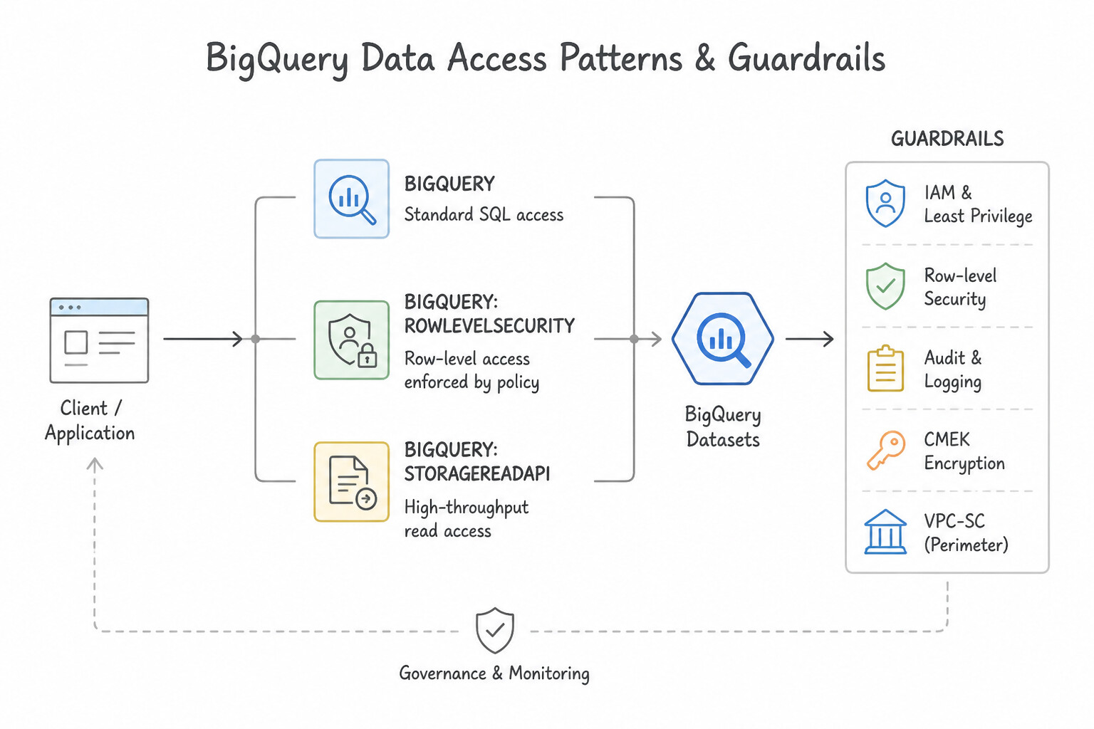
• Restricting Row Access for Multi-Tenant Data: Use Configure BigQuery row-level security policies to filter results based on the user's account. Row-level security dynamically filters data in a single table based on the user's identity. (Avoid alternative: Separating tables increases overhead and violates the single-table requirement.)
• High-Throughput Read for Custom ML Models: Use Modify the training application to use the BigQuery Storage Read API. The BigQuery Storage Read API enables high-throughput, parallel reads directly from BigQuery storage using gRPC, ideal for ML workloads. (Avoid alternative: JDBC drivers are designed for standard application connectivity and BI, not for the high-throughput parallel scanning required for ML training.)
• Accelerating Aggregates on Streaming Data: Use Create a BigQuery materialized view that computes the required aggregates. Materialized views pre-compute aggregates and automatically sync with streaming data, reducing scan costs and latency. (Avoid alternative: Scheduled queries introduce data staleness and do not meet the real-time requirement.)

Key Takeaways (3.2d)

• IAM roles generally control access at the resource level (dataset or table), not the data row level.
• Authorized Views act as wrappers to restrict data but can create management overhead if one is needed for every user.
• Row-Level Security (RLS) is the standard method for filtering specific rows based on user identity in a single table.
• Avoid exporting data to Cloud Storage if you require low-latency access for downstream processing; read directly from the source when possible.

Quick Decision Cheat Sheet (Subsection 3.2)

Further Reading (Subsection 3.2)

• Nested and repeated columns — This page explains how to create and query nested and repeated columns in BigQuery, which is the standard way to handle denormalized one-to-many relationships.
• BigQuery best practices: Schema design — Guidelines on designing schemas for performance, specifically recommending denormalization to optimize query execution.
• Introduction to clustered tables — Documentation explaining how clustering works, when to use it, and how it differs from partitioning.
• Introduction to partitioned tables — Official Google Cloud documentation explaining how partitioned tables work, when to use them, and the benefits of partition pruning for cost and performance.
• Querying partitioned tables — Details on how to write queries that leverage partition pruning effectively.
• Optimizing Schema for Performance — Discusses best practices for schema design, specifically highlighting the reduction of joins via denormalization.

Subsection 3.3: Using a data lake

Section 3: Storing the Data

The Big Picture

A modern Google Cloud data lake centers on Cloud Storage (gs://) unified with BigLake, Dataplex, and Dataproc. Teams migrating from on-premises Hadoop or building ad-hoc object lakes hit three major architectural traps:

1. The Persistent HDFS & Stateful Cluster Anti-Pattern (3.3a, 3.3b): Running a 24/7 persistent Dataproc cluster storing data on local Compute Engine HDFS disks means you pay for idle CPUs all night, cannot scale compute down without losing HDFS replication blocks, and lose all data if the cluster is deleted. On Google Cloud, Cloud Storage (gs://) via the Cloud Storage Connector replaces HDFS as the persistent storage layer; metadata lives in Dataproc Metastore, and compute runs on ephemeral job-scoped Dataproc clusters or Dataproc Serverless for Spark!
2. Fine-Grained Object ACLs vs. Uniform Bucket-Level Access & BigLake (3.3a): Mixing legacy POSIX/object ACLs with Cloud IAM on a data lake bucket makes auditing who can read sensitive files nearly impossible. Google Cloud best practice mandates enabling Uniform Bucket-Level Access (UBLA) so 100% of bucket access is governed deterministically by Cloud IAM, and wrapping lake files in BigLake Tables (via a Cloud Resource Connection service account) so analysts never need direct raw GCS bucket access and receive full Row-Level and Column-Level Security.
3. Unpartitioned CSV Lake Scans (3.3b, 3.3c): Storing raw uncompressed CSVs in a flat bucket forces Spark and BigQuery External Tables to scan every byte on every query. Organizing Cloud Storage in a Hive-Partitioned directory layout (gs://lake/sales/dt=2026-10-13/region=US/part-001.parquet) using compressed Apache Parquet / Apache Iceberg enables automatic partition predicate pushdown and column pruning.

Consideration 3.3a: Managing the lake (configuring data discovery, access, and cost controls)

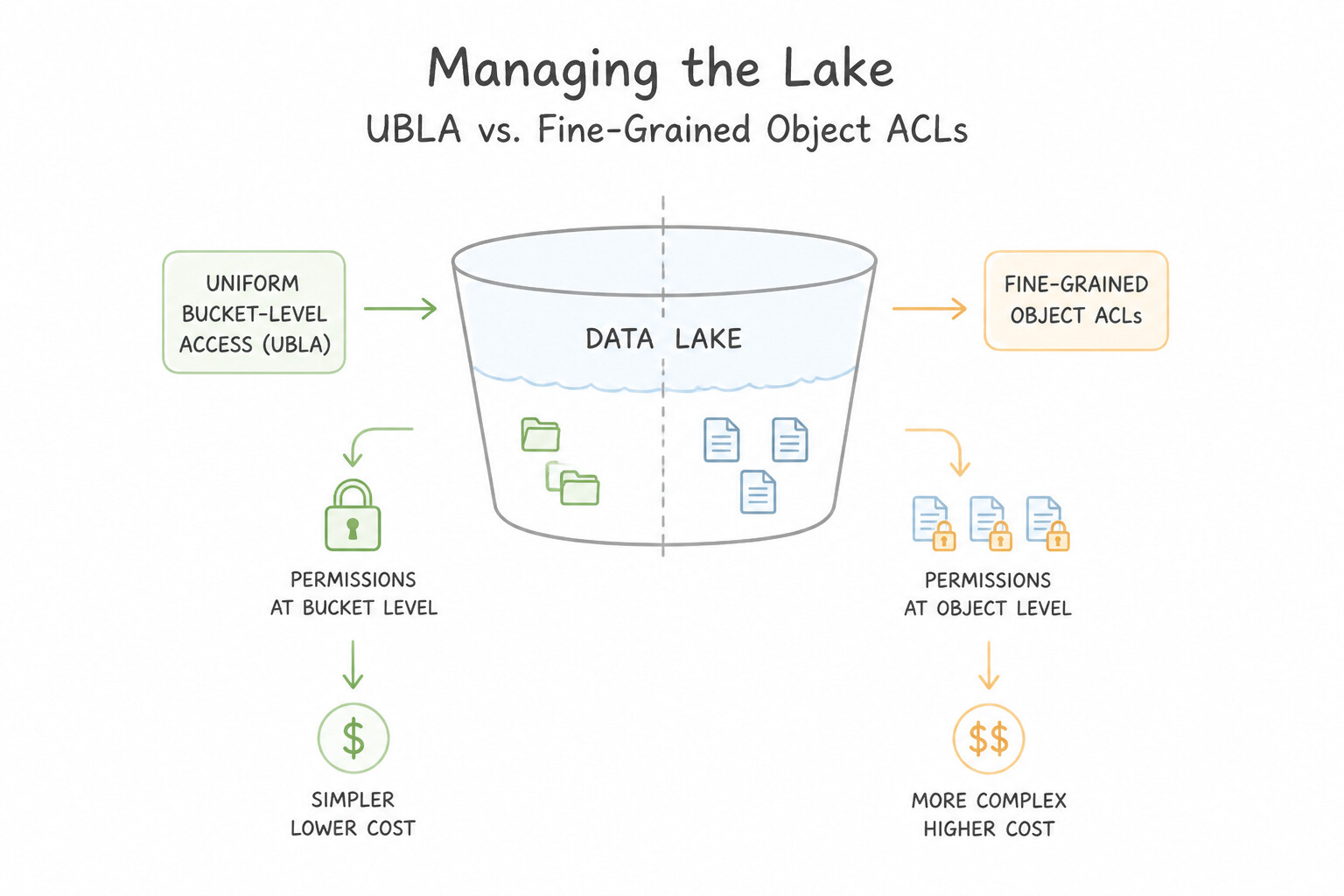
Govern your Cloud Storage data lake with unified IAM and BigLake virtualization:

• Uniform Bucket-Level Access (UBLA) vs. Fine-Grained Object ACLs:
• Always enable Uniform Bucket-Level Access on data lake buckets. It disables legacy per-object ACLs so access is evaluated strictly through Cloud IAM and IAM Conditions (and is required for VPC Service Controls, Workforce Identity Federation, and Folder-level IAM inheritance).
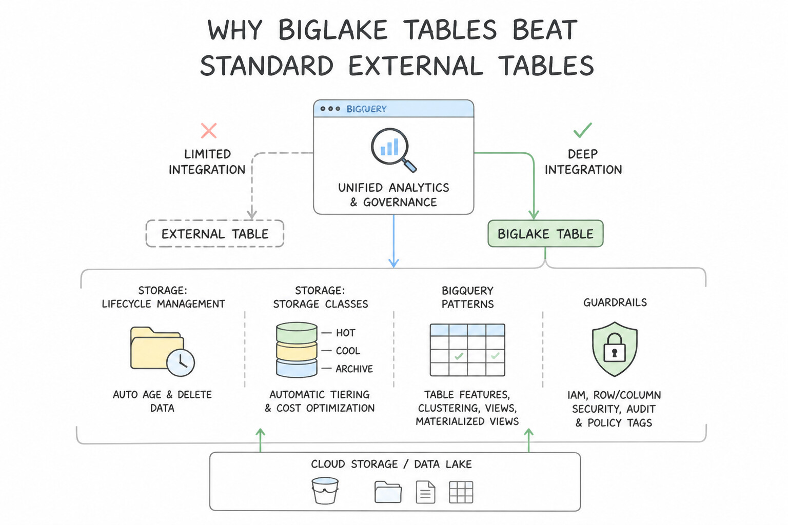
• Why BigLake Tables Beat Standard External Tables:
• With a standard BigQuery External Table, the querying user must be granted both BigQuery permissions and direct roles/storage.objectViewer on the underlying Cloud Storage bucket—meaning the user can bypass BigQuery views and download the raw Parquet files directly via gcloud storage cp!
• With a BigLake Table, you create a Cloud Resource Connection whose dedicated Service Account is the only identity granted roles/storage.objectViewer on the GCS bucket. Users query the BigLake table through BigQuery with zero direct GCS permissions, and BigQuery enforces Row-Level Security (Row Access Policies), Column-Level Security (Policy Tags), and Dynamic Data Masking on the GCS Parquet/CSV/ORC/Iceberg files!
• BigLake Metadata Caching for Million-File Lakes:
• Listing millions of GCS objects at query startup adds seconds of latency. Enabling BigLake Metadata Caching (max_staleness = INTERVAL 30 MINUTE) caches object names, partition keys, and Parquet column min/max statistics in BigQuery memory, dramatically accelerating partition and file pruning.

Key Implementation Patterns

• Cost Optimization for Log Archival: Use Configure Object Lifecycle Management on the bucket. Add a rule with an Age condition of 30 days to change the storage class to Archive Storage. Add a second rule with an Age condition of 3 years to delete the objects. Object Lifecycle Management automates storage class transitions and deletion based on object age, which minimizes costs and operational overhead.
• Securing Sensitive Columns in Data Lake Files: Use Create a taxonomy and policy tags in Data Catalog. Apply a policy tag to the SSN column in the BigQuery schema. Grant the HR team the Fine-Grained Reader role on the policy tag. Data Catalog Policy Tags provide the standard mechanism for implementing column-level security in BigQuery.
• Unified Data Governance Across Projects: Use Create a Dataplex lake. Create zones within the lake for Sales, Raw, and Curated data. Add the existing Cloud Storage buckets as assets to these zones. Dataplex allows you to map distributed physical storage into logical Lakes and Zones for centralized governance and quality monitoring without moving data.

Key Takeaways (3.3a)

• Use Object Lifecycle Management to automate cost optimization for Cloud Storage.
• Choose the appropriate storage class (Standard, Nearline, Coldline, Archive) based on access frequency and retention period.
• Avoid custom scripts for standard maintenance tasks when a native platform feature exists.
• Archive Storage is the most cost-effective option for long-term retention of rarely accessed data.

Consideration 3.3b: Processing data

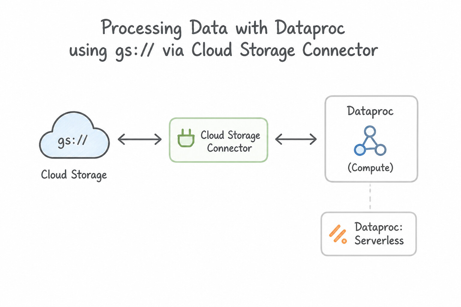
Master the decoupled Spark/Hadoop architecture on Google Cloud:

• Replace HDFS with gs:// (Cloud Storage Connector):
• Only use local HDFS / Local SSDs on Dataproc for ephemeral intermediate shuffle files (spark.local.dir). Store all input and output tables in gs:// buckets.
• Avoid the Hadoop FileOutputCommitter rename bottleneck on object storage (since rename in object storage is a copy+delete operation) by using the modern Cloud Storage connector output committers or writing to BigLake / Apache Iceberg.
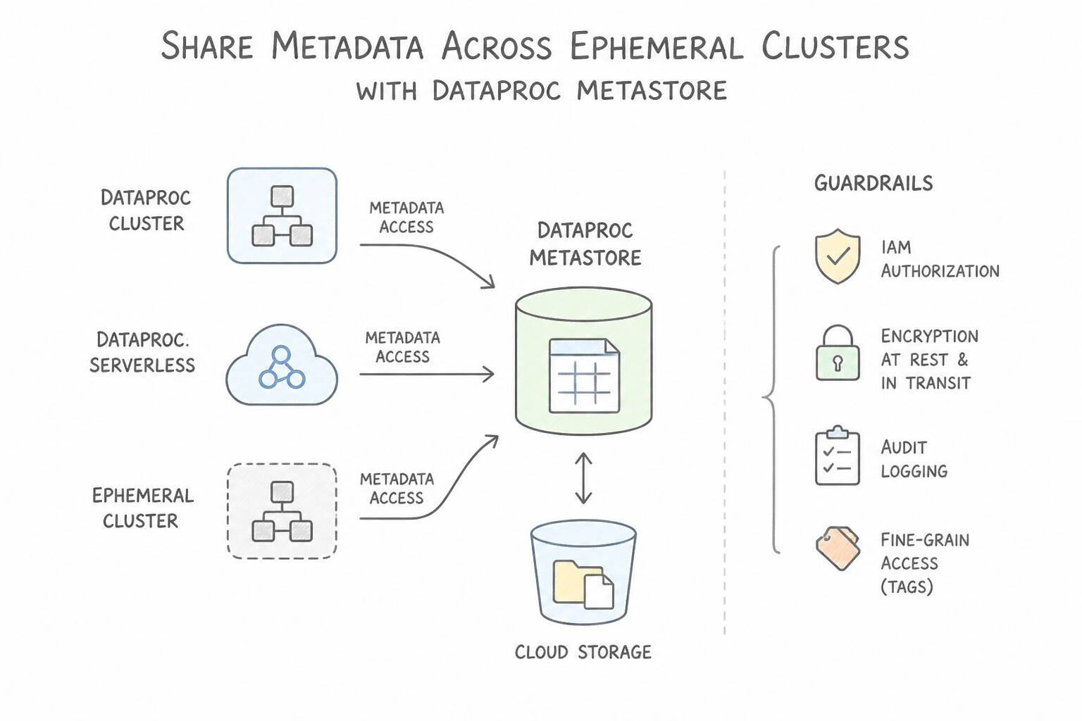
• Share Metadata Across Ephemeral Clusters with Dataproc Metastore:
• When ephemeral Dataproc clusters spin up for a 30-minute Spark job and then delete themselves, any local MySQL Hive metastore on the master node is destroyed with the cluster. Use Dataproc Metastore (a fully managed, highly available Apache Hive Metastore service) or BigLake Metastore so multiple ephemeral Dataproc clusters, Dataproc Serverless jobs, and Trino/Presto engines share a single persistent catalog!
• Choosing the Right Dataproc Deployment Mode:
• Dataproc Serverless for Spark: Submit PySpark/Spark batch jobs or interactive notebooks with zero cluster management—Google provisions and autoscales compute automatically per job.
• Dataproc on Compute Engine (Ephemeral Clusters): Full control over VM machine types, custom initialization actions, YARN tuning, and open-source Hadoop components (HBase, Presto, Flink, Zeppelin).
• Dataproc on GKE: Best when your engineering organization already standardizes on Google Kubernetes Engine (GKE) and wants to run Spark jobs as Kubernetes pods sharing existing GKE node pools and CI/CD tooling.

Key Implementation Patterns

• Decoupling Storage and Compute in Hadoop Migrations: Use Modify the jobs to use the Cloud Storage connector to read and write data to Cloud Storage buckets. Cloud Storage decouples storage from compute, allowing data access even when the cluster is deleted. (Avoid alternative: HDFS runs on the cluster nodes; shutting down the cluster makes HDFS data inaccessible.)
• Serverless Spark for Variable Workloads: Use Submit the Spark workload to Dataproc Serverless as a batch job. Dataproc Serverless runs Spark batches without requiring you to manage clusters, scaling policies, or OS patching. (Avoid alternative: Rewriting Spark jobs to Apache Beam for Dataflow is unnecessary extra work when Dataproc Serverless supports Spark natively.)
• Optimizing Spot Instance Usage for Batch Processing: Use Enable Enhanced Flexibility Mode (EFM) to store shuffle data on primary workers. EFM decouples shuffle data from secondary workers, preventing data loss when Spot VMs are reclaimed. (Avoid alternative: Standard VMs are much more expensive than Spot VMs and do not satisfy the cost-minimization requirement.)

Key Takeaways (3.3b)

• Decoupling: Separate compute (Dataproc) from storage (Cloud Storage) to enable ephemeral clusters.
• Cost Optimization: Shutting down idle clusters saves significantly on Compute Engine costs.
• Connector: The Cloud Storage connector allows Hadoop applications to use GCS seamlessly without major code rewrites.
• Dataproc Serverless removes the need to manage clusters or configure auto-scaling for Spark batch workloads.

Consideration 3.3c: Monitoring the data lake

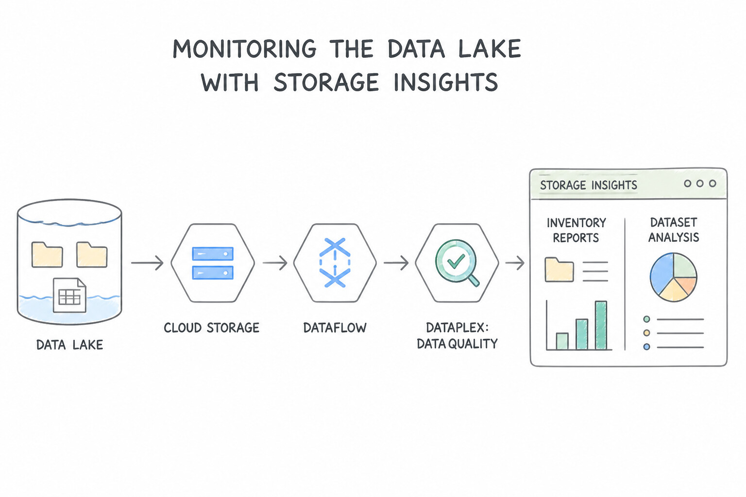
Keep a multi-petabyte data lake observable, performant, and compliant:

• Storage Insights (Inventory Reports & Dataset Analysis): Instead of running expensive gcloud storage ls -r list operations across 500 million objects (which incurs Class A operation fees and takes hours), enable Cloud Storage Insights Inventory Reports to export daily Parquet/CSV metadata inventories (bucket, object_name, size, storage_class, last_modified, etag) directly into BigQuery for cost and stale-data analysis.
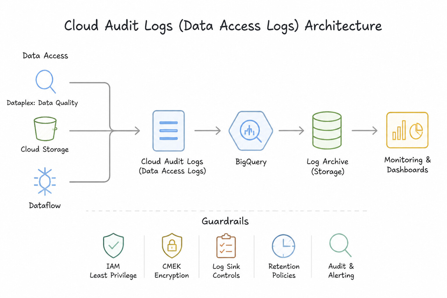
• Cloud Audit Logs (Data Access Logs): Admin Activity audit logs are always on and free (tracking bucket creation/IAM changes). To monitor who read or wrote specific sensitive objects in a data lake bucket, explicitly enable DATA_READ and DATA_WRITE Data Access Audit Logs on Cloud Storage (or monitor access centrally through BigLake query audit logs!).
• Diagnosing Small-File Syndrome & Throughput Limits: Thousands of tiny <1 MB files in a GCS lake degrade Spark and BigQuery External Table scan speeds due to per-object HTTP open overhead. Monitor object size distributions via Storage Insights / Dataplex and run periodic compaction jobs (or use BigLake Managed Tables for Apache Iceberg with automatic file compaction) to consolidate files into optimal 128 MB – 512 MB Parquet blocks.

Key Implementation Patterns

• Automating Data Quality Checks in Data Lakes: Use Create a Dataplex Data Quality task. Define the validation rules in a YAML specification file and schedule the task to run on the Dataplex entities. Dataplex Data Quality allows you to automate validation rules using simple YAML configuration files without writing custom code.
• Auditing Object Deletion: Use Enable Data Access audit logs for the Cloud Storage API. Data Access audit logs capture object-level operations (reads/writes) and must be explicitly enabled for Cloud Storage. (Avoid alternative: Cloud Monitoring provides aggregated metrics on usage and performance, not identity-based audit trails for specific actions.)

Key Takeaways (3.3c)

• Dataplex is the go-to service for managing, monitoring, and governing distributed data lakes in Google Cloud.
• Dataplex Auto Data Quality uses YAML configuration to validate data without custom code.
• Avoid writing custom pipelines (Dataflow/Cloud Functions) for standard tasks when a managed service exists.
• Validating data in place (in GCS) is preferable to moving bad data into a warehouse (BigQuery) before checking it.

Quick Decision Cheat Sheet (Subsection 3.3)

Further Reading (Subsection 3.3)

• Object Lifecycle Management — Documentation on how to configure lifecycle rules, including supported actions like SetStorageClass and Delete, and conditions like Age.
• Storage Classes — Overview of different storage classes, their pricing models, and intended use cases.
• Introduction to column-level security — Provides an overview of how BigQuery uses Data Catalog policy tags to restrict access to specific columns.
• Restrict access with column-level security — Detailed guide on setting up taxonomies, policy tags, and IAM roles to enforce column-level security.
• Dataplex Overview — Provides a high-level overview of Dataplex capabilities, including logical organization of lakes and zones.
• Dataplex Terminology — Explains the definitions of Lake, Zone, and Asset and how they map to physical resources.

Subsection 3.4: Designing for a data platform

Section 3: Storing the Data

The Big Picture

As an enterprise scales across dozens of business domains (Retail, Banking, Logistics, Marketing, HR), data platform architecture hits an organizational wall:

• If a single Central IT team owns every pipeline, bucket, and dataset in one monolithic project, the central team becomes a 6-month bottleneck because they don't understand domain-specific schemas.
• Conversely, if every business unit builds its own isolated project with zero central standards, the enterprise fragments into ungoverned data silos with inconsistent IAM policies, duplicated data, and zero cross-domain discoverability.

Subsection 3.4 tests how you solve this paradox on Google Cloud by building an intelligent Data Fabric / Federated Data Mesh Platform using Dataplex, Dataplex Catalog, BigQuery, and Cloud Storage—achieving decentralized domain ownership with centralized federated governance.

Consideration 3.4a: Building a data platform using Google Cloud tools (e.g., Dataplex, Dataplex Catalog, BigQuery, Cloud Storage)

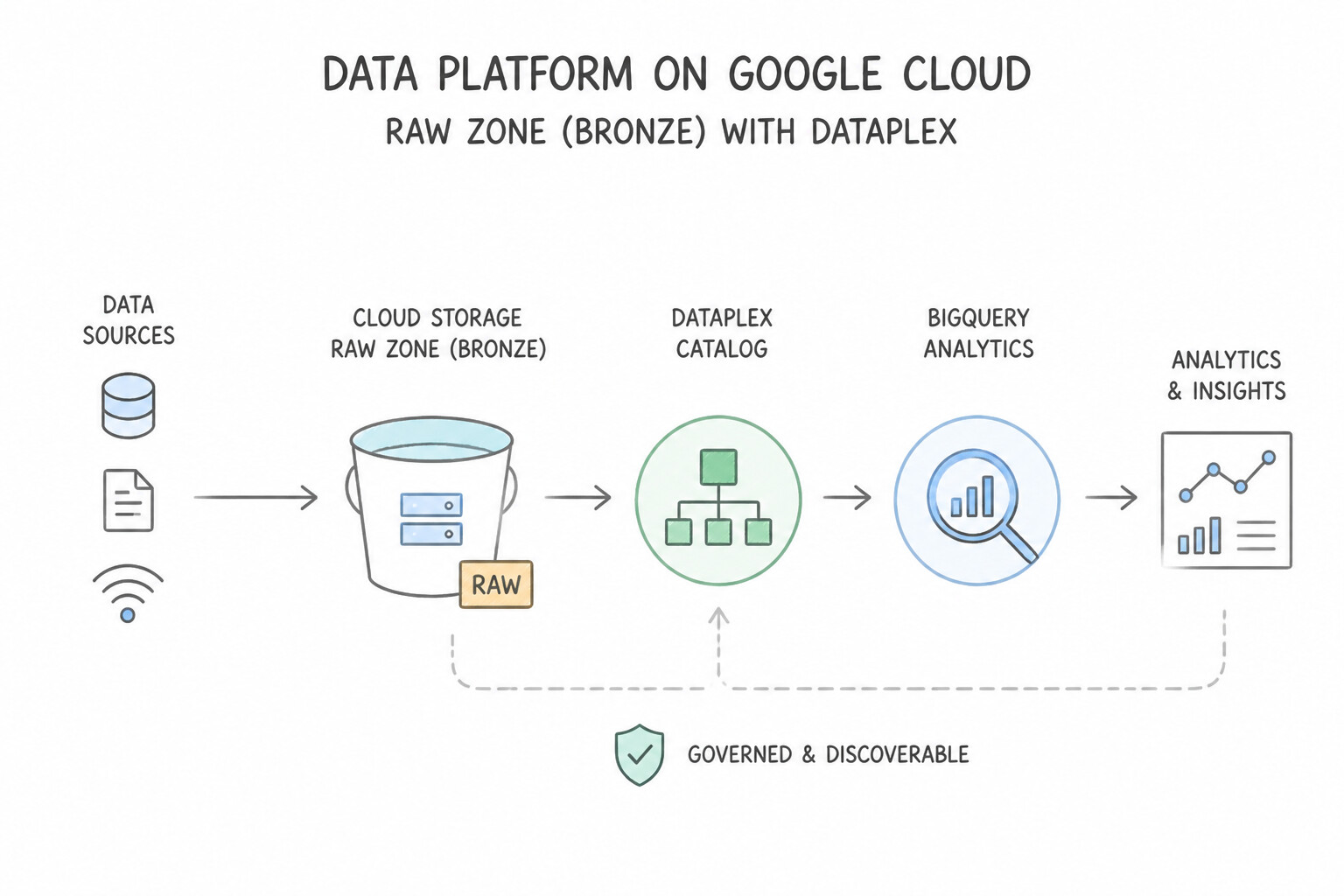
Master the exact three-level logical hierarchy of Google Cloud Dataplex (Lake → Zone → Asset):

1. Dataplex Lake (Business Domain Construct):
2. Represents a logical business domain or organizational unit (e.g., retail-sales-lake, supply-chain-lake, finance-lake).
3. A single Dataplex Lake can unify physical storage resources spanning multiple Google Cloud projects without moving or copying a single byte of data!
4. Dataplex Zone (Raw Zone vs. Curated Zone):
5. A sub-grouping within a Lake representing data readiness, environment, or consumer contract:
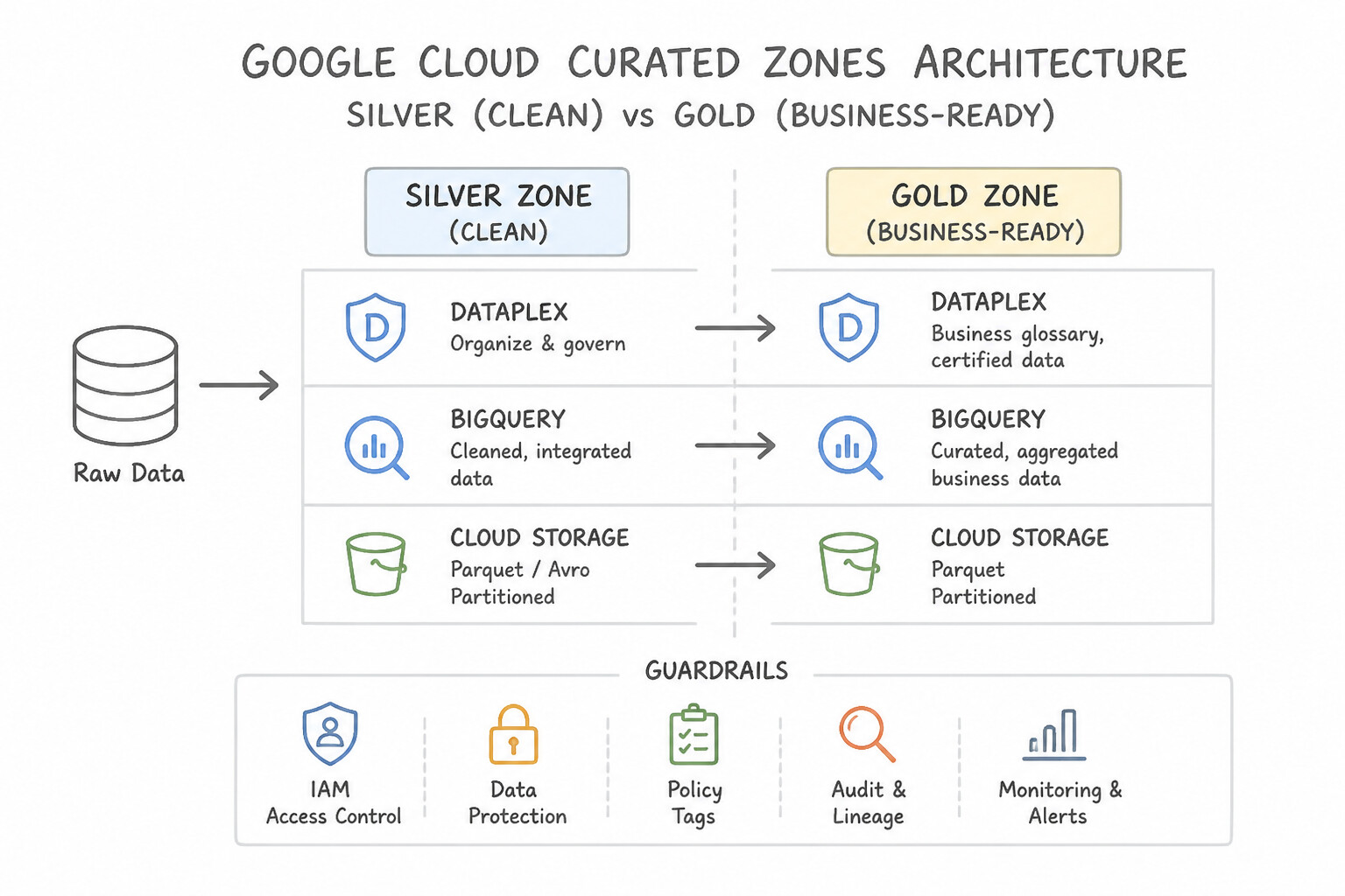
6. Raw Zone (Bronze): Accepts any data format (unstructured files, raw CSVs, JSON logs, images) in Cloud Storage buckets or BigQuery datasets with flexible schema rules.
7. Curated Zone (Silver / Gold): Enforces strict formatting and schema governance—only formatted structured/columnar data (Parquet, Avro, ORC in Cloud Storage, or BigQuery datasets) that conforms to compatible Hive partition structures and schema evolution rules is permitted!
8. Dataplex Asset (Physical Storage Mapping):
9. Maps an existing Cloud Storage bucket or BigQuery dataset (even if hosted in a separate domain project) into a Zone.
10. Once attached as an Asset, Dataplex automatically discovers tables, registers schemas into Dataplex Catalog / BigQuery / Dataproc Metastore, and propagates Zone-level IAM permissions down to the physical bucket/dataset!

Key Implementation Patterns

• Implementing a Data Mesh Architecture: Use Use Dataplex. Create a Lake for each business domain. Within each Lake, create Zones for data readiness levels. Add the existing Cloud Storage buckets and BigQuery datasets as Assets. Dataplex allows you to logically organize data into Lakes (domains) and Zones (readiness) without physical movement, enabling a Data Mesh architecture.
• Unified Security for Data Lakes (BigLake): Use Create a BigLake table that references the Cloud Storage files. Apply the row-level security policies directly to the BigLake table. BigLake extends BigQuery's fine-grained security features, such as row-level security, to data stored externally in Cloud Storage.
• Automating Data Quality Checks: Use Define data quality rules in a YAML file and schedule a Dataplex data quality task. Dataplex AutoDQ uses declarative YAML configuration and is serverless. (Avoid alternative: Dataflow requires writing custom code, which violates the scenario requirements.)

Key Takeaways (3.4a)

• Dataplex is the primary tool for implementing Data Mesh on Google Cloud.
• Lakes map to organizational domains (Sales, Finance).
• Zones map to data readiness (Raw, Curated) or restrictions.
• Dataplex manages data in place; it does not require physical data migration.

Consideration 3.4b: Building a federated governance model for distributed data systems

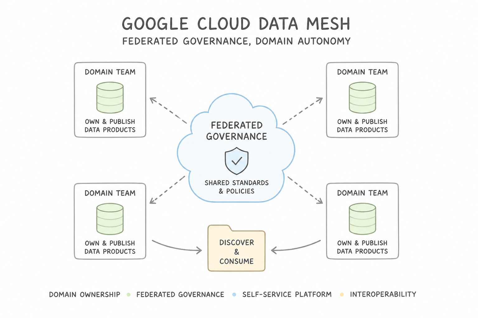
When a workload scenario requires for a Data Mesh or Federated Data Governance across independent business units:

• The Core Principles of a Google Cloud Data Mesh (3.4b):
• Domain-Oriented Ownership: Each business unit (e.g., Marketing, Logistics, Risk) manages its own pipelines and stores its own physical Cloud Storage buckets and BigQuery datasets in its own domain Google Cloud project, mapped to its own Dataplex Lake.
• Data as a Product: Domains publish clean, documented, SLA-backed tables in their Curated Zone (Gold) and share them across domains via Analytics Hub or Dataplex permissions.
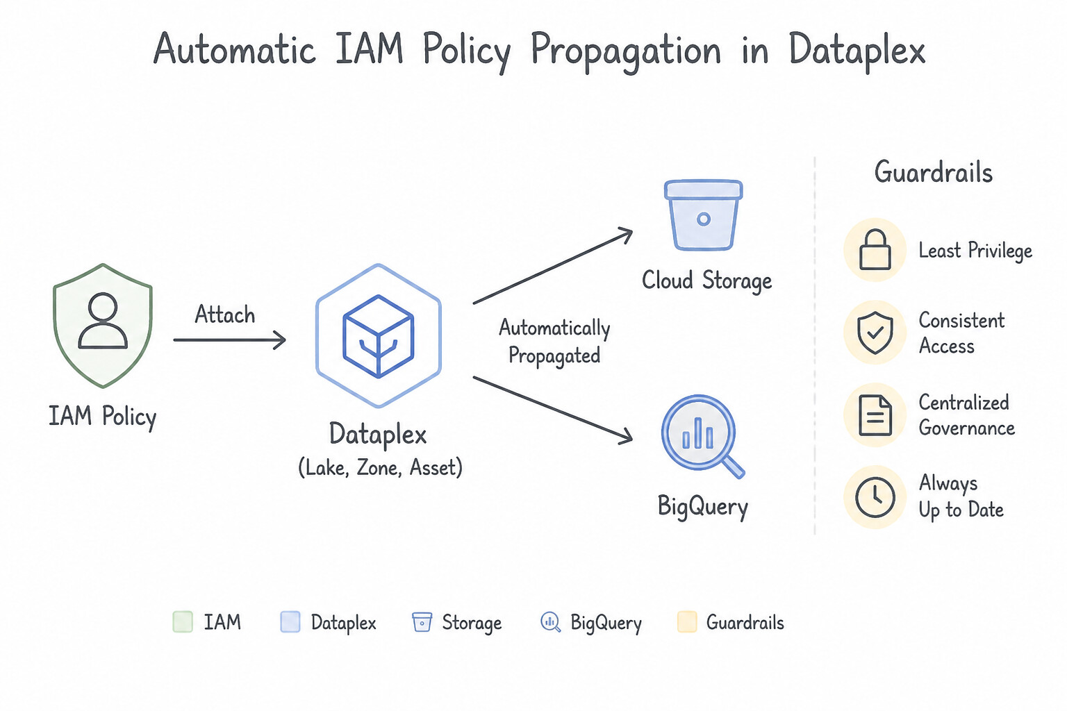
• Centralized Federated Governance: A central Governance/Security team defines organization-wide Dataplex Catalog Taxonomies & Policy Tags (High-PII, Financial-Restricted), Aspect Types / Tag Templates (Data Steward, Quality Tier, Retention Class), and Dataplex Auto Data Quality rules—which apply uniformly across every domain's Lake and Zone regardless of which underlying project holds the physical bytes!
• Automatic IAM Policy Propagation in Dataplex:
• Instead of manually managing separate IAM bindings on 50 Cloud Storage buckets and 80 BigQuery datasets across 12 projects, grant roles/dataplex.dataReader or roles/dataplex.dataWriter at the Dataplex Lake or Zone level—Dataplex automatically propagates the corresponding physical storage.objectViewer and bigquery.dataViewer permissions to every underlying Asset in that Zone!

Key Implementation Patterns

• Logical Data Organization without Migration: Use Create Dataplex Lakes for each business domain. Configure Zones within the Lakes and map the existing resources as Assets. Dataplex allows you to map existing physical resources (buckets, datasets) to logical constructs (Lakes, Zones) for governance without moving data.
• Zero-Copy Data Sharing Across Organizations: Use Create an exchange in Analytics Hub. Publish a listing containing the dataset and grant access to the suppliers. Analytics Hub enables secure, governed, zero-copy data sharing across organizations via exchanges and listings.
• Fine-Grained Access Control via Taxonomy: Use Create a taxonomy in Data Catalog (Dataplex) with policy tags. Apply these tags to the PII columns and grant the Fine-Grained Reader role to authorized users. Policy tags allow you to define sensitivity centrally and enforce column-level access control across multiple projects using IAM roles.

Key Takeaways (3.4b)

• Dataplex enables a Data Mesh architecture on Google Cloud.
• Dataplex Lakes and Zones provide logical organization for distributed data without physical movement.
• Assets in Dataplex map to existing Cloud Storage buckets and BigQuery datasets.
• Use Dataplex for unified governance, security, and discovery across disparate projects.

Quick Decision Cheat Sheet (Subsection 3.4)

Further Reading (Subsection 3.4)

• Dataplex terminology — This page defines the core concepts of Dataplex, including Lakes, Zones, and Assets, and how they map to physical resources.
• Dataplex Universal Catalog — Describes how to use Dataplex to implement a domain-oriented data mesh architecture.
• Introduction to BigLake external tables — Provides an overview of BigLake capabilities, specifically highlighting fine-grained access control for data lakes.
• Row-level security — Explains how row-level security works in BigQuery and its compatibility with BigLake tables.
• Dataplex Data Quality Overview — Describes how Dataplex allows you to define data quality rules using YAML and execute them as serverless jobs.
• Dataplex Overview — Provides the official definition of Dataplex, Lakes, Zones, and Assets, explaining how they fit into a data mesh architecture.

Book TOC · Previous · Chapter 3 of 6 · Next