Book TOC · Previous · Chapter 5 of 6 · Next

Chapter 5: DataOps: FinOps Resource Optimization, CI/CD Repeatability, Observability & Fault Mitigation

Subsections Covered: 5.1, 5.2, 5.3, 5.4, 5.5 (15 Considerations · 30 Custom Visual Diagrams)

Chapter Focus: BigQuery Editions (Autoscaling Slots: Standard/Enterprise/Enterprise Plus) vs. on-demand, physical vs. logical storage billing, Dataflow straggler/hotkey debugging, INFORMATION_SCHEMA diagnostics, and DR failover.

Subsection 5.1: Optimizing resources

Section 5: Maintaining and Automating Data Workloads

The Big Picture

Section 5 (Maintaining and automating data workloads, ~18% in Google Cloud architectures) tests how you run production data systems efficiently at scale. Subsection 5.1 focuses on FinOps and resource optimization across Dataproc, Dataflow, BigQuery, and Cloud Composer. Three costly mistakes dominate production scenarios:

1. The 24/7 Persistent Cluster Anti-Pattern (5.1a, 5.1c): Keeping a 50-node Dataproc cluster running 24 hours a day to execute three 45-minute Spark batch jobs means paying for 21+ hours of idle VMs daily, plus managing noisy-neighbor contention when jobs overlap. Switching to ephemeral job-scoped Dataproc clusters (automated via Dataproc Workflow Templates) or Dataproc Serverless for Spark reading/writing directly to Cloud Storage (gs://) cuts compute costs by 70–85% while guaranteeing strict per-job isolation.
2. Misconfiguring Spot / Preemptible Workers & Shuffle Disks (5.1a, 5.1b): Adding Spot (Preemptible) VMs as primary Dataproc workers causes HDFS block corruption and YARN master instability when instances are preempted. Spot VMs must be added exclusively as Secondary Workers (--num-secondary-workers) (which run compute only and zero HDFS DataNodes!), paired with Enhanced Flexibility Mode (EFM) or Local SSDs so shuffle data survives worker preemption without full stage recomputation.
3. Unbounded Autoscaling & Missing Cost Attribution (5.1a, 5.1b): Launching Dataflow pipelines without --maxNumWorkers or running multi-department queries without Resource Labels (labels) and Cloud Billing Export to BigQuery makes FinOps chargeback and cost ceiling enforcement impossible.

Consideration 5.1a: Minimizing costs per required business need for data

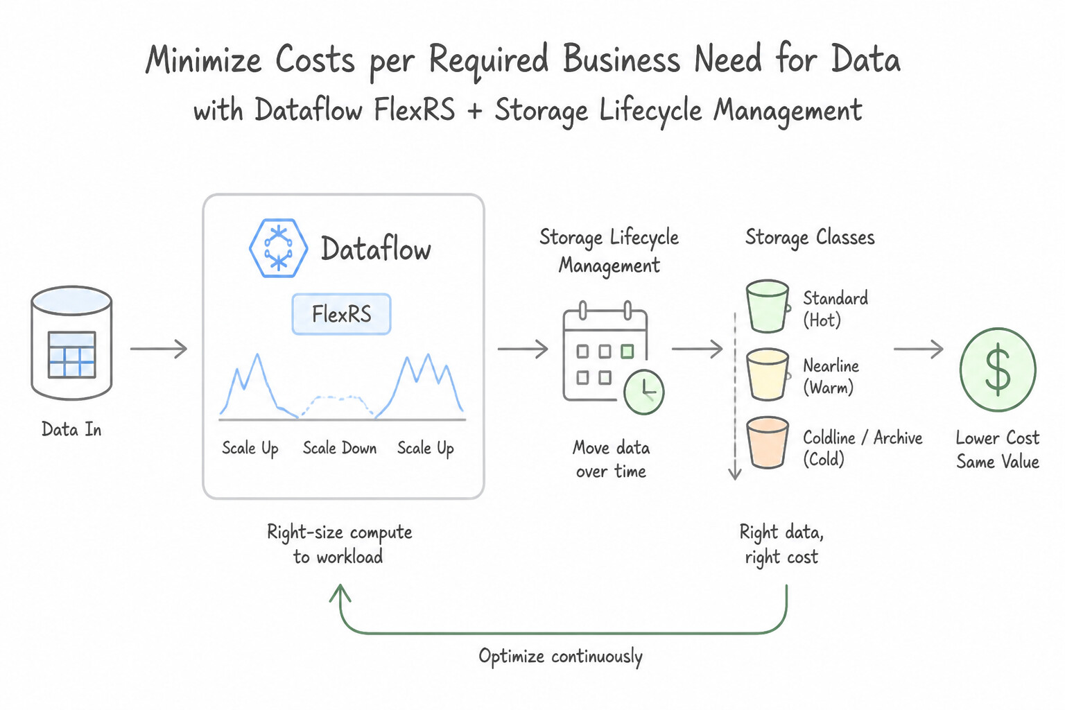
Match every workload's latency tolerance to the most cost-effective execution tier:

• Dataflow Flexible Resource Scheduling (FlexRS):
• When a batch Dataflow pipeline is not time-critical (e.g., a nightly/weekly log processing job that just needs to finish within a 6-hour window), enable Dataflow FlexRS. FlexRS queues the job for up to 6 hours to wait for discounted Spot/Preemptible capacity paired with standard VMs, reducing batch compute costs by ~40%!
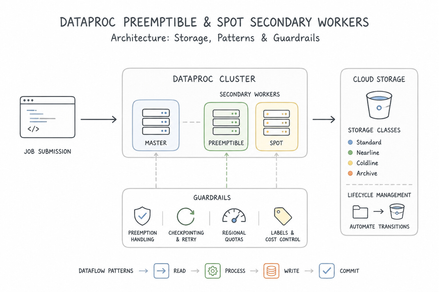
• Dataproc Preemptible / Spot Secondary Workers:
• Add Spot VMs (Preemptible VMs) as Secondary Workers to reduce per-core Spark/Hadoop compute costs by 60–91%.
• Golden Rule: Secondary workers in Dataproc never store HDFS data (they are compute-only YARN nodes). Keep primary workers on standard non-preemptible VMs so YARN ApplicationMasters and HDFS NameNodes remain stable.
• Granular Cost Attribution (Resource Labels + Cloud Billing Export to BigQuery):
• Whenever an production scenarios asks how to track, allocate, or charge back BigQuery, Dataflow, and Dataproc costs across 10 internal departments sharing projects → attach Labels (key:value pairs like department:finance, env:prod) to every BigQuery job (configuration.labels), Dataflow job, and Dataproc cluster, and analyze the Detailed Usage Cost Billing Export in BigQuery!

Key Implementation Patterns

• Optimizing Cloud Storage Costs via Lifecycle Management: Use Configure an Object Lifecycle Management rule to change the storage class to Nearline after 30 days and to Archive after 90 days. Transitioning data to Nearline after 30 days and Archive after 90 days aligns storage costs with the decreasing access frequency.
• Cost-Efficient Batch Processing with Dataflow FlexRS: Use Submit the job using Dataflow Flexible Resource Scheduling (FlexRS). FlexRS minimizes costs by delaying execution to an optimal time and using a mix of standard and preemptible resources. (Avoid alternative: Standard VMs run at full price and do not take advantage of the flexible scheduling window to reduce costs.)
• Reducing BigQuery Analysis Costs with Partitioning and Clustering: Use Create a new table that is partitioned by the timestamp column and clustered by device_id. Partitioning by date and clustering by ID minimizes data scanned for queries filtering on both fields. (Avoid alternative: Partitioning by device_id is not feasible due to the limit of 4,000 partitions per table.)

Key Takeaways (5.1a)

• Match storage classes to access patterns: Standard for frequent, Nearline for monthly, Coldline for quarterly, Archive for yearly.
• Use Object Lifecycle Management to automate cost savings by moving aging data to colder storage tiers.
• Always respect data retention compliance requirements before considering deletion for cost savings.
• FlexRS is ideal for batch jobs that are not time-critical and can be delayed by a few hours.

Consideration 5.1b: Ensuring enough resources for business-critical data processes

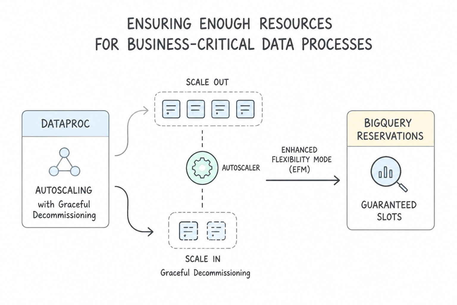
Prevent resource starvation and shuffle bottlenecks on mission-critical jobs:

• Dataproc Autoscaling with Graceful Decommissioning & Enhanced Flexibility Mode (EFM):
• When scaling down a Dataproc cluster (or when Spot secondary workers are preempted), abrupt node removal kills active Spark executors and forces expensive re-computation of map-stage shuffle files stored on that worker's local disk.
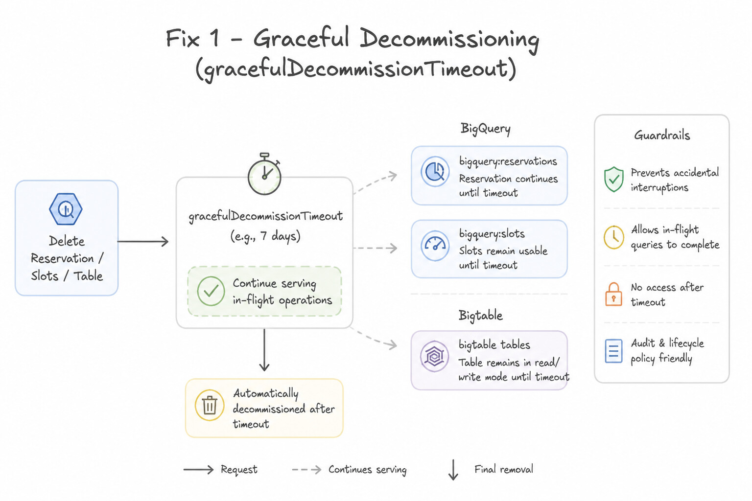
• Fix 1 — Graceful Decommissioning (gracefulDecommissionTimeout): Configure a graceful decommission timeout in the Dataproc Autoscaling Policy so YARN waits for running tasks and shuffle migrations to complete before terminating the node.
• Fix 2 — Enhanced Flexibility Mode (EFM): Stores intermediate Spark shuffle data only on Primary Workers (or external shuffle storage) so secondary Spot workers remain 100% stateless and can be preempted at any second without triggering stage retries!
• Fix 3 — Local SSDs for Shuffle-Bound Spark Jobs: If Spark stages bottleneck on disk I/O during massive groupByKey/join shuffles, attach Local SSDs to worker nodes for high-IOPS scratch space.
• Dataflow Streaming Engine, Dataflow Prime & @Setup Reuse:
• Enable Streaming Engine (offloads window state and shuffle from worker VM disks/CPUs to a managed Google backend, allowing faster, smoother autoscaling with smaller worker VMs).
• Enable Dataflow Prime with Vertical Autoscaling when pipeline steps suffer from unexpected OutOfMemoryError spikes—Dataflow Prime automatically scales worker RAM vertically while Horizontal Autoscaling adjusts worker count!

Key Implementation Patterns

• BigQuery Workload Isolation: Use Purchase BigQuery slots. Create a reservation for the dashboards and assign the project to this reservation. Reservations allow you to isolate and guarantee compute capacity (slots) for critical workloads, preventing resource contention.
• Bigtable Workload Separation: Use Add a second cluster to the Bigtable instance. Create separate app profiles with single-cluster routing to direct transactional traffic to the primary cluster and analytics traffic to the new cluster. Use replication and app profiles with single-cluster routing to physically isolate transactional and analytics workloads onto separate clusters.
• Dataproc High Availability for Critical Jobs: Use Configure the cluster to use Standard VMs for primary workers and Spot VMs for secondary workers. Primary workers host HDFS data and must remain stable using Standard VMs; secondary workers are compute-only and can safely use Spot VMs to save costs.

Key Takeaways (5.1b)

• Slots are the unit of compute in BigQuery.
• Reservations are used to isolate workloads and guarantee capacity for critical business processes.
• On-demand pricing uses a shared pool of resources, which can lead to performance variance under heavy load.
• Batch priority reduces cost or resource pressure but is unsuitable for interactive or SLA-driven workloads.

Consideration 5.1c: Deciding between persistent or job-based data clusters (e.g., Dataproc)

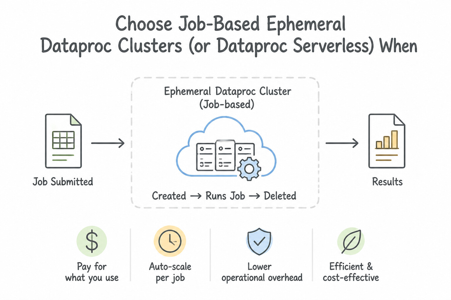
This is a classic PDE tie-breaker question. Memorize the exact comparison:

• Choose Job-Based Ephemeral Dataproc Clusters (or Dataproc Serverless) When:
• Workloads are scheduled batch jobs (hourly, nightly, weekly) or event-triggered pipelines.
• Strict cost attribution or security/dependency isolation per job or per team is required (each job runs on its own clean cluster with its own Service Account and Python/Jar versions, then deletes the cluster immediately upon completion).
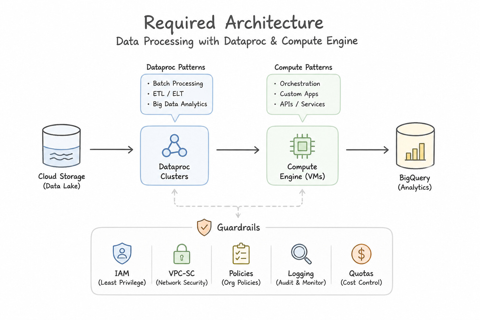
• Required Architecture: Store data in Cloud Storage (gs://), store Hive table schemas in Dataproc Metastore, and orchestrate creation → execution → deletion via Dataproc Workflow Templates or Cloud Composer.
• Choose Persistent Dataproc Clusters (with Autoscaling) Only When:
• Running 24/7 continuous Spark Streaming jobs where cluster spin-up latency (60–90 seconds) cannot be tolerated, OR supporting a large team of data scientists running interactive ad-hoc Jupyter/Zeppelin sessions continuously throughout the workday where instant sub-second cluster attachment is mandatory.

Key Implementation Patterns

• Cost Optimization for Infrequent Batch Jobs: Use Use a Dataproc Workflow Template to create a cluster, run the job, and delete the cluster. Ephemeral clusters run only for the duration of the job, saving costs on idle resources. (Avoid alternative: Preemptible VMs reduce hourly rates but do not solve the cost inefficiency of running an idle cluster for 22 hours.)
• Low-Latency Interactive Analytics: Use Create a persistent Dataproc cluster that runs during working hours. Persistent clusters eliminate the startup latency of provisioning resources, making them ideal for interactive notebook usage. (Avoid alternative: Automating the creation of a cluster on-demand still results in wait times while the infrastructure initializes.)

Key Takeaways (5.1c)

• Identify Idle Time: If a resource is idle for significant periods, look for ways to shut it down.
• Ephemeral is Cost-Effective: For periodic batch jobs, creating a cluster on-demand (ephemeral) is almost always cheaper than a persistent one.
• Automate Lifecycle: Use tools like Dataproc Workflow Templates to automate the creation and deletion of resources.
• Use persistent clusters for interactive workloads (notebooks, ad-hoc queries) to avoid startup latency.

Quick Decision Cheat Sheet (Subsection 5.1)

Further Reading (Subsection 5.1)

• Storage classes — Documentation detailing the different storage classes, their intended use cases, and pricing models.
• Object Lifecycle Management — Guide on how to configure lifecycle rules to automatically transition or expire objects.
• Use Flexible Resource Scheduling (FlexRS) — This page explains how FlexRS helps reduce batch processing costs by using advanced scheduling techniques and preemptible VMs.
• Introduction to partitioned tables — Explains how partitioning works, its benefits for query performance and cost, and how partition pruning reduces bytes scanned.
• Introduction to clustered tables — Details how clustering works to sort data and how it complements partitioning to further optimize queries.
• Introduction to Reservations — Overview of how BigQuery Reservations work, including the hierarchy of reservations and assignments.

Subsection 5.2: Designing automation and repeatability

Section 5: Maintaining and Automating Data Workloads

The Big Picture

An automated pipeline is only production-grade if it is repeatable (idempotent)—meaning that if a network glitch causes Tuesday's 02:00 AM run to fail halfway through, re-running Tuesday's job (or running a 30-day historical backfill) produces the exact same target table state without duplicating rows or overwriting Wednesday's data. Subsection 5.2 tests how you engineer repeatable Cloud Composer (Apache Airflow) DAGs and automated schedules:

1. The CURRENT_DATE() & WRITE_APPEND Non-Idempotency Bug (5.2a, 5.2b): If an Airflow task runs INSERT INTO sales_summary SELECT ... WHERE dt = CURRENT_DATE() with WRITE_APPEND, re-running a failed job from 3 days ago processes today's date instead of 3 days ago, and appends duplicate rows on every retry! Repeatable Airflow DAGs parameterize queries with the logical execution date ({{ ds }} / {{ data_interval_start }}) and write to the specific target partition (sales_summary${{ ds_nodash }}) using WRITE_TRUNCATE (or an atomic MERGE).
2. Blocking Worker Slots with Synchronous Sensors & Top-Level Code (5.2a): Writing bigquery.Client() or SecretManagerServiceClient() calls at the top level of a DAG .py file executes those network RPCs every 30 seconds inside the Airflow Scheduler's DAG parser—bringing the entire Cloud Composer environment to its knees! Equally fatal is running 50 GCSObjectExistenceSensor tasks in default poke mode, which consumes 50 worker slots sleeping in while loops and deadlocks all downstream tasks.

Consideration 5.2a: Creating directed acyclic graphs (DAGs) for Cloud Composer

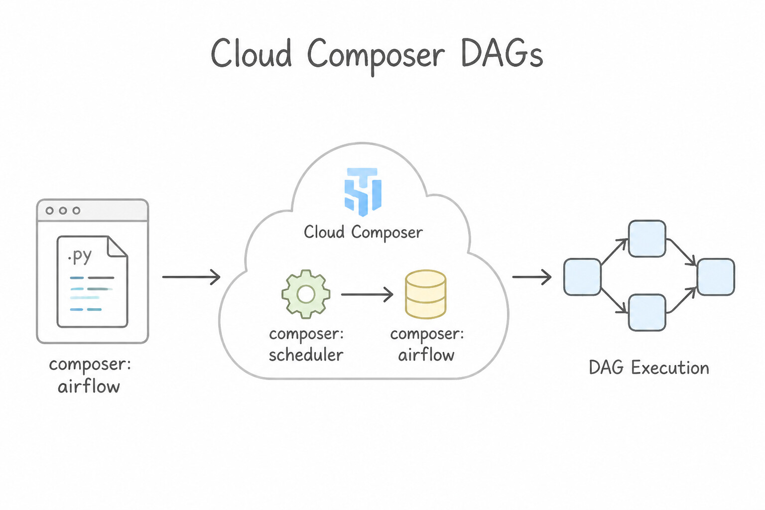
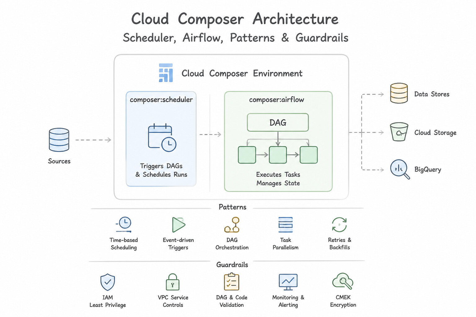
Follow these 5 ironclad rules when authoring and troubleshooting Cloud Composer DAGs in production:

1. Keep Top-Level DAG Code 100% Free of Network/DB Calls:
2. The Airflow Scheduler re-parses every .py file in the dags/ bucket every ~30 seconds. Never put Variable.get() (unless inside a Jinja template '{{ var.value.my_var }}'), Secret Manager calls, or BigQuery queries at the top level of the Python file! Put all runtime calls inside operator parameters or inside a task's execution function.
3. Use Native Google Cloud Operators Over Custom PythonOperator Loops:
4. Use BigQueryInsertJobOperator, DataflowStartFlexTemplateOperator, DataprocInstantiateWorkflowTemplateOperator, and GCSToBigQueryOperator so compute runs in the managed service, not inside the Composer GKE worker pod.
5. Never Pass Data Payloads Through XCom:
6. Airflow XCom (cross-communication) is stored in the Cloud Composer metadata database (Cloud SQL) and is strictly for tiny metadata strings (like a job_id or a gs://bucket/path/output.parquet URI). Never pass multi-megabyte DataFrames or query results via XCom—write intermediate data to Cloud Storage or a BigQuery staging table and pass only the URI/table reference in XCom!
7. Use Deferrable Operators (deferrable=True) or mode="reschedule" for Sensors:
8. Default mode="poke" holds onto a worker slot while sleeping between checks. Switching to deferrable=True (uses the async Airflow Triggerer component) or mode="reschedule" frees the worker slot between checks so other tasks never deadlock.
9. Guarantee Cleanup with TriggerRule.ALL_DONE:
10. If a DAG creates a temporary resource (Step 1) → runs a Spark job (Step 2) → deletes the temporary resource (Step 3), set trigger_rule="all_done" on Step 3 so the cleanup task executes even if Step 2 fails!

Key Implementation Patterns

• Optimizing DAG Parsing Speed: Use Refactor the DAG to perform the SQL query within a task and use dynamic task mapping to generate the downstream tasks. Moving the heavy query into a task prevents it from running during the frequent DAG parsing loop. (Avoid alternative: Scaling resources does not fix the inefficient code causing the high load.)
• Data Sharing Between Tasks: Use Use XComs to push the partition ID in the first task and pull the value in the second task. XComs are the native Airflow feature for passing small metadata (like a partition ID string) between tasks. (Avoid alternative: Global variables do not persist across distributed workers in Airflow; tasks cannot share state this way.)
• Implementing Conditional Workflows: Use Use the BranchPythonOperator to return the task ID of the next task to execute based on the file extension. BranchPythonOperator allows you to dynamically determine which task to run next based on custom Python logic, enabling conditional branching.

Key Takeaways (5.2a)

• Avoid top-level code in DAG files; it runs on every scheduler heartbeat.
• Move heavy computations or external calls (API/DB) into Operators or Hooks.
• Use Dynamic Task Mapping to generate tasks based on runtime data.
• Keep DAG parsing time low to ensure scheduler health.

Consideration 5.2b: Scheduling and orchestrating jobs in a repeatable way

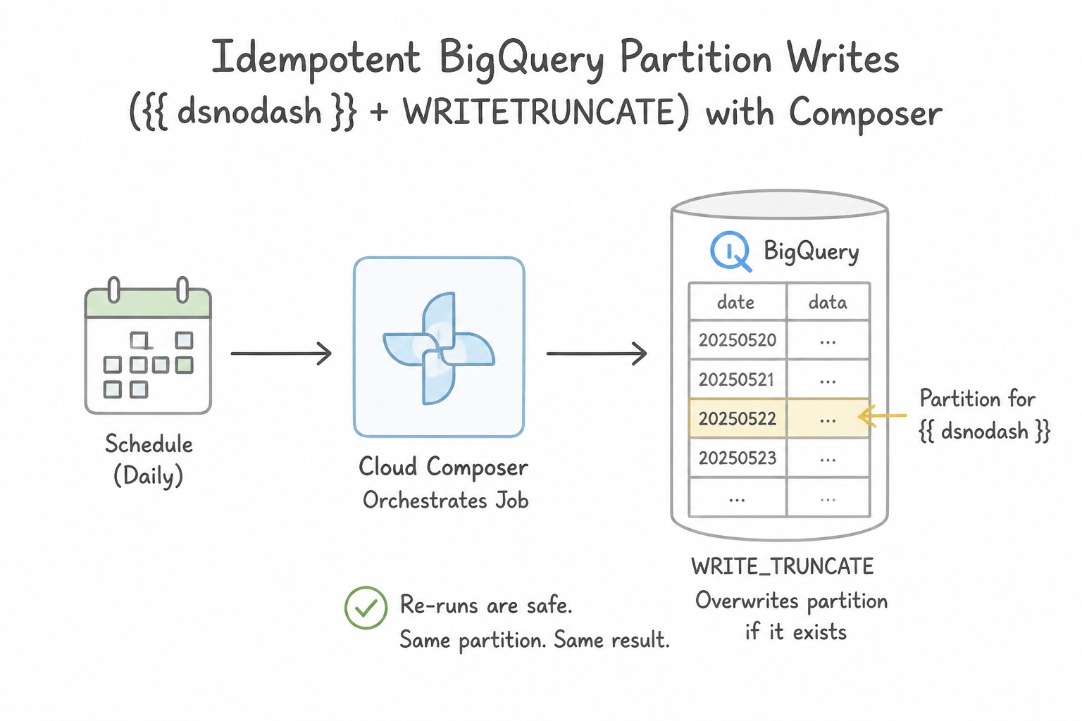
Repeatable orchestration ensures that any task or entire DAG run can be cleared and re-executed safely:

• Idempotent BigQuery Partition Writes ({{ ds_nodash }} + WRITE_TRUNCATE):
• Bind every scheduled batch load or transformation to Airflow's logical execution date ({{ ds }} = YYYY-MM-DD, {{ ds_nodash }} = YYYYMMDD).
• Target the exact partition decorator project.dataset.table${{ ds_nodash }} with write_disposition="WRITE_TRUNCATE". Whether the task runs once, retries 3 times after a timeout, or runs as part of a 90-day catchup=True backfill, each date partition is atomically overwritten with exact, duplicate-free data!
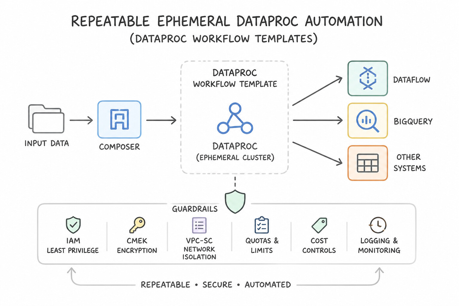
• Repeatable Ephemeral Dataproc Automation (Dataproc Workflow Templates):
• Define a parameterized Dataproc Workflow Template in YAML/Terraform that specifies the managed cluster spec (machine types, Spot workers, initialization actions), the ordered sequence of PySpark/Hive jobs, and automatic cluster teardown. Trigger it repeatably from Cloud Scheduler (via Cloud Workflows/Functions) or Cloud Composer (DataprocInstantiateWorkflowTemplateOperator).
• Event-Driven vs. Polling Schedules:
• If upstream partner files arrive at unpredictable times throughout the day, replace fixed cron schedules + long-running sensors with Event-Driven Orchestration: configure Eventarc (or a GCS Pub/Sub notification + Cloud Function/Workflows) on google.cloud.storage.object.v1.finalize to trigger the Cloud Composer DAG via the Airflow REST API (dagRuns endpoint) passing the exact gs:// object URI in conf!

Key Implementation Patterns

• Orchestrating Heterogeneous Services: Use Develop a Directed Acyclic Graph (DAG) in Cloud Composer to orchestrate the tasks. Cloud Composer (Apache Airflow) is the correct tool for orchestrating complex, multi-step workflows with strict dependencies and scheduling. (Avoid alternative: Cloud Functions has execution time limits and is not designed to orchestrate long-running dependent workflows.)
• Serverless Workflow Chaining: Use Define the orchestration logic in a YAML file and deploy it to Cloud Workflows. Cloud Workflows is serverless, scales to zero, and is optimized for low-latency microservice orchestration. (Avoid alternative: Cloud Composer is designed for batch data pipelines, does not scale to zero, and has higher latency overhead.)
• Lightweight API Scheduling: Use Create a Cloud Scheduler job configured with a cron schedule to invoke the Cloud Function via HTTP. Cloud Scheduler is the standard, managed service for triggering Cloud Functions on a time-based schedule. (Avoid alternative: Managing a VM solely for a cron job adds unnecessary maintenance and cost.)

Key Takeaways (5.2b)

• Cloud Composer (Apache Airflow) is the go-to service for complex workflow orchestration involving dependencies.
• Cloud Scheduler is for simple time-based triggering, not managing multi-step workflows.
• Cloud Functions are for short-lived, event-driven code and have timeouts that make them unsuitable for waiting on long-running jobs.
• Avoid using unmanaged VMs (Cron) when a managed service is available.

Quick Decision Cheat Sheet (Subsection 5.2)

Further Reading (Subsection 5.2)

• Best practices for writing DAGs — Official Airflow documentation explaining why top-level Python code should be avoided and its impact on performance.
• Optimize environment performance and costs — Google Cloud documentation regarding DAG coding standards to prevent high scheduler CPU usage.
• Airflow Concepts - XComs — Official documentation describing how XComs let tasks exchange messages and the limitations on data size.
• Cloud Composer - Writing DAGs — Google Cloud documentation on best practices for writing DAGs in Composer, including data handling.
• Branching in Airflow — Documentation explaining how branching works in Airflow, specifically highlighting the BranchPythonOperator usage.
• Cloud Composer Overview — Explains that Cloud Composer is a fully managed workflow orchestration service built on Apache Airflow.

Subsection 5.3: Organizing workloads based on business requirements

Section 5: Maintaining and Automating Data Workloads

The Big Picture

As an organization's BigQuery usage matures from a single team to hundreds of analysts, data scientists, and automated ETL pipelines, running everything in a single unisolated pool breaks down in two ways:

1. The Noisy-Neighbor Slot Starvation Problem (5.3a): If the Data Science team launches an exploratory 50-join ML feature query at 8:59 AM in the same slot pool used by the CEO's 9:00 AM revenue dashboard, the exploratory query consumes thousands of slots and causes the executive dashboard to hang. BigQuery Reservations (Workload Management) solve this by carving slot capacity into isolated Reservations (prod-bi, elt-pipelines, adhoc-ds) assigned to specific Folders or Projects—while still allowing idle slots to be borrowed instantaneously across reservations whenever a pool is quiet!
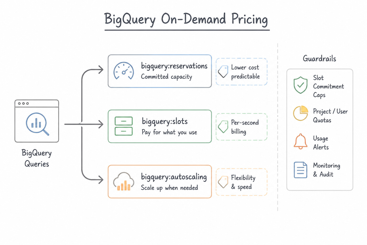
2. Overpaying for Spiky Workloads vs. Starving Background Batch Jobs (5.3a, 5.3b): Under legacy flat-rate commitments, you had to provision enough fixed slots for your highest 1-hour peak and pay for them 24/7. BigQuery Editions (Standard, Enterprise, Enterprise Plus) introduce Slot Autoscaling between a configurable baseline (minimum guaranteed slots) and max_reservation_size (cost ceiling), billed per second. Pairing Reservations with INTERACTIVE vs. BATCH query priorities ensures urgent user queries execute immediately while non-urgent background jobs queue gracefully and run on idle capacity.

Consideration 5.3a: Capacity management (e.g., BigQuery Editions and reservations)

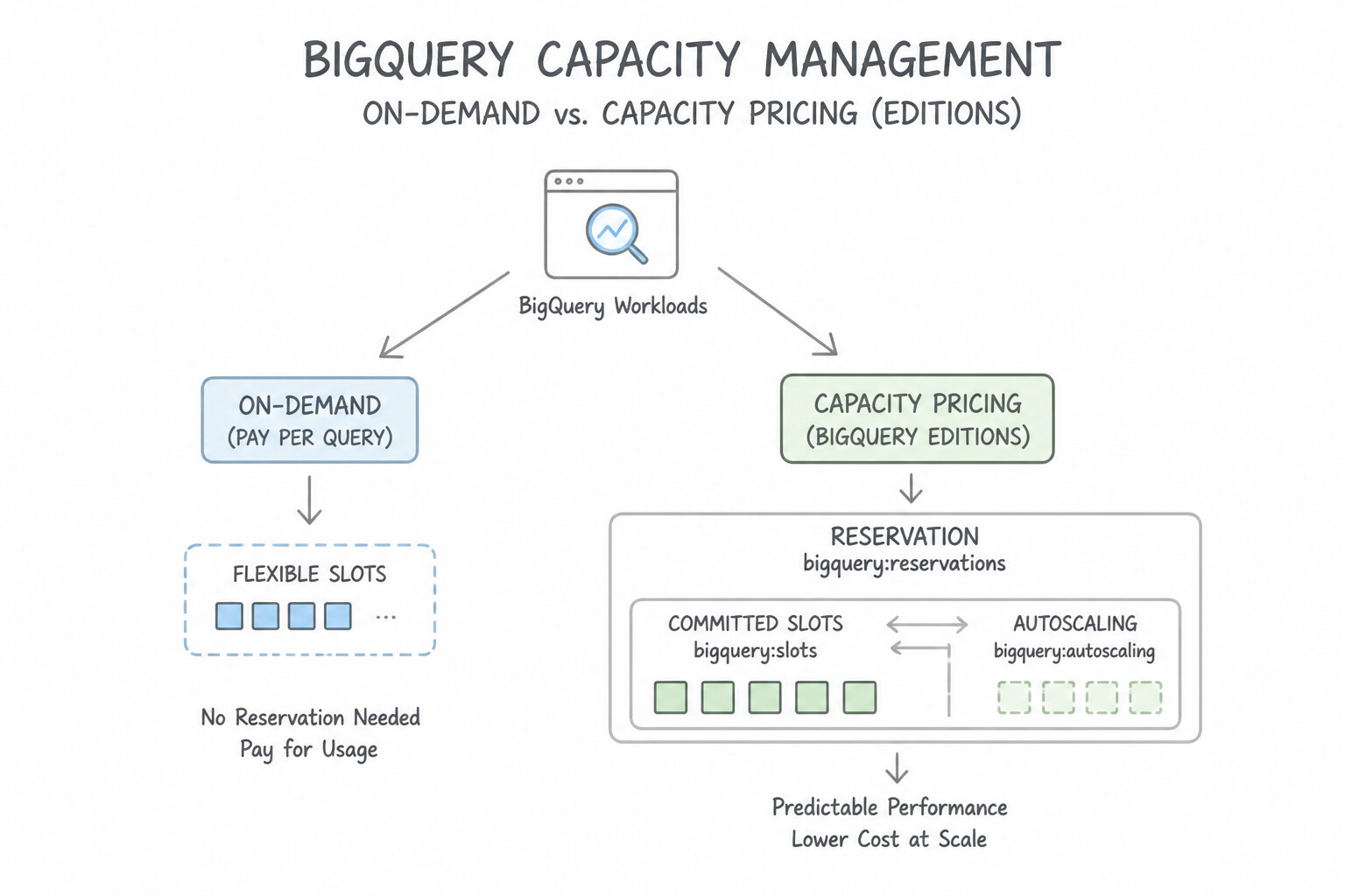
Master the BigQuery Workload Management hierarchy (Administration Project → Capacity Commitment / Edition → Reservation → Assignment):

• On-Demand vs. Capacity Pricing (BigQuery Editions):
• On-Demand Pricing: Charges per TiB of data scanned (\$6.25/TiB after the first 1 TiB/month free), up to a shared project burst limit (~2,000 slots). Best for spiky, low-volume, or unpredictable early-stage workloads where queries are well-partitioned/clustered.
• BigQuery Editions (Standard, Enterprise, Enterprise Plus): Pay for compute capacity (slot-hours, billed per second in increments of 50–100 slots) rather than bytes scanned!
• Standard Edition: Entry-level autoscaling slots (capped max slots, basic security, 99.9% SLA).
• Enterprise Edition: Unlimited slot autoscaling, optional 1-year/3-year baseline commitments, BI Engine inclusion, BigQuery ML advanced models, Row/Column-Level Security, Autoscale down to 0 baseline, 99.99% SLA.
• Enterprise Plus Edition: Adds Customer-Managed Encryption Keys (CMEK), FedRAMP / HIPAA / ITAR compliance controls, and Managed Cross-Region Disaster Recovery (DR).
• Baseline Slots, Max Reservation Size & Idle Slot Sharing:
• Every Reservation in Enterprise/Enterprise Plus defines baseline slots (always warm and dedicated to that reservation) and max_slots (baseline + autoscale).
• Idle Slot Sharing: By default (ignore_idle_slots = false), if Reservation A (prod-bi) has 500 baseline slots sitting idle at 2:00 AM, Reservation B (nightly-elt) can borrow those 500 idle slots for free—and the exact millisecond a prod-bi query arrives, BigQuery preempts the borrowed slots and returns them immediately to prod-bi!
• Hard Cost Cap for Sandbox/Ad-Hoc Teams: To strictly cap a Data Science sandbox's spend so they can never autoscale beyond 200 slots and never pay per-TiB on-demand fees, assign their project to a Reservation with baseline = 0, max_slots = 200, and ignore_idle_slots = true (or allow idle slot borrowing if free unused baseline exists).
• Assigning None to Force On-Demand Billing: If an entire Organization folder is assigned to an Enterprise Reservation, you can still exclude one specific project back to On-Demand (per-TiB) billing by creating an explicit Assignment for that project set to None!

Key Implementation Patterns

• Workload Isolation for Mission-Critical Dashboards: Use Create a dedicated reservation for the dashboard project. Assign the dashboard project to this reservation. Reservations isolate compute capacity (slots) for specific projects, guaranteeing performance for critical workloads.
• Optimizing for Idle Capacity Sharing: Use Create an administration project with a Capacity Commitment. Create a reservation for each department. Assign each department's project to its corresponding reservation. Centralized commitments with specific reservations allow idle slots to be shared automatically by default.
• Cost Capping with BigQuery Editions: Use Create a reservation with a low baseline. Set the maximum reservation size to a specific value that aligns with your budget. Setting the maximum reservation size limits the total slots available during autoscaling, strictly capping the potential cost.

Key Takeaways (5.3a)

• BigQuery Slots are the unit of compute capacity.
• Reservations allow you to allocate specific amounts of slots to specific workloads for isolation.
• Assignments link projects to reservations to enforce which compute pool they use.
• Isolating critical workloads (like dashboards) from heavy ad-hoc workloads prevents performance degradation.

Consideration 5.3b: Interactive or batch query jobs

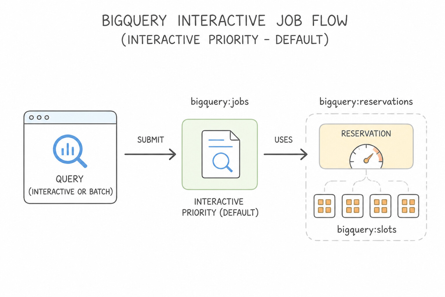
Classify every BigQuery SQL workload into INTERACTIVE or BATCH priority:

• INTERACTIVE Priority (Default):
• Executes the query as soon as possible.
• Counts against concurrent interactive query rate limits.
• Use for: live user-facing dashboards, Looker/Looker Studio queries, and interactive analyst investigation.
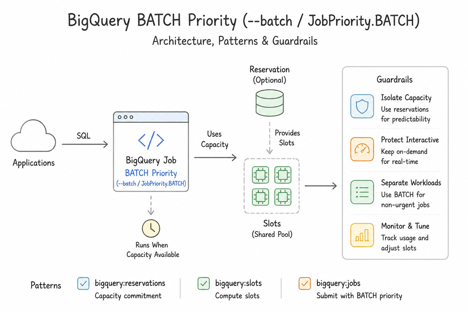
• BATCH Priority (--batch / JobPriority.BATCH):
• BigQuery queues the query on behalf of the user and starts execution as soon as idle slot resources become available in the reservation (or within 24 hours at most).
• Advantages:
• Prevents non-urgent scheduled reports or historical backfill queries from competing with live INTERACTIVE dashboards for slots!
• Does not count toward the concurrent interactive query quota limit.
• Under On-Demand pricing, batch queries still cost the same per-TiB scanned (unless using dedicated reservations where they soak up already-paid idle baseline slots!).

Key Implementation Patterns

• BigQuery Workload Isolation with Reservations: Use Enable BigQuery Reservations. Create a reservation with dedicated slots and assign the BI team's project to this reservation. BigQuery Reservations allow you to isolate workloads by assigning dedicated slots to specific projects, guaranteeing performance.
• Optimizing Costs for Non-Urgent ETL: Use Submit the query job with the priority set to BATCH. Batch priority moves the job to a queue that uses idle resources, avoiding contention with interactive queries. (Avoid alternative: Buying more slots incurs extra cost and does not specifically address the scheduling priority.)

Key Takeaways (5.3b)

• Slots are the unit of compute in BigQuery.
• Reservations are used to isolate workloads and guarantee capacity.
• Interactive jobs are for immediate user-facing tasks; Batch jobs are for deferred processing.
• Assignments map projects to specific reservations to enforce resource limits and guarantees.

Quick Decision Cheat Sheet (Subsection 5.3)

Further Reading (Subsection 5.3)

• Introduction to Reservations — This page explains the fundamental concepts of BigQuery Reservations, including slots, capacity commitments, and assignments. Read the section on 'Assignments' to understand how to map projects to reserved capacity.
• Workload Management using Slots — Explains the concept of slots as the unit of computational capacity in BigQuery.
• Introduction to BigQuery Editions — Overview of BigQuery Editions, including the differences between Standard, Enterprise, and Enterprise Plus, and how slot-based pricing works.
• Work with reservations — Documentation on creating and managing reservations, specifically explaining how to set baseline slots and maximum reservation sizes for autoscaling.
• Interactive and batch query jobs — Documentation explaining the difference between interactive and batch query priorities and how to specify them.

Subsection 5.4: Monitoring and troubleshooting processes

Section 5: Maintaining and Automating Data Workloads

The Big Picture

When a real-time fraud pipeline lags by 40 minutes, a Bigtable cluster's P99 read latency jumps from 6ms to 450ms, or a BigQuery reservation hits 100% slot saturation, guessing and randomly adding VMs wastes money and rarely fixes the root cause. Subsection 5.4 tests diagnostic precision: knowing the exact metric, system view, or diagnostic visualizer for every Google Cloud data service:

1. Diagnosing Dataflow Streaming Backlog vs. System Lag (5.4a, 5.4c): In Dataflow, System Lag (system_lag) measures the maximum duration an item of data has been awaiting processing inside the pipeline, while Data Watermark Age tracks the age of the oldest unprocessed event. If CPU utilization across all workers is at 85% and System Lag is climbing, the job is compute-bound (increase --maxNumWorkers). If only one worker's CPU is at 100% while 19 others are at 5%, you have a Hot Key (use Combine.perKey with .withHotKeyFanout()). If CPU is <10% across all workers while System Lag climbs, the pipeline is blocked waiting on an external synchronous RPC or sink quota!
2. Diagnosing BigQuery via INFORMATION_SCHEMA & Admin Resource Charts (5.4a, 5.4b, 5.4d): Never parse raw text logs to find slow queries or reservation bottlenecks. Query region-us.INFORMATION_SCHEMA.JOBS_BY_PROJECT (or JOBS_BY_ORGANIZATION) for total_slot_ms, total_bytes_billed, and bi_engine_statistics, and inspect INFORMATION_SCHEMA.RESERVATIONS_TIMELINE alongside the BigQuery Admin Panel (Capacity Management & Resource Charts) to spot slot contention (concurrency > available slots).
3. Diagnosing Bigtable with Key Visualizer (5.4a, 5.4c): When a Cloud Bigtable cluster slows down despite low average CPU (<30%), open Key Visualizer—a bright horizontal ribbon reveals a hot row key range (monotonic timestamp prefix or celebrity key) hitting a single tablet!

Consideration 5.4a: Observability of data processes (e.g., Cloud Monitoring, Cloud Logging, BigQuery admin panel)

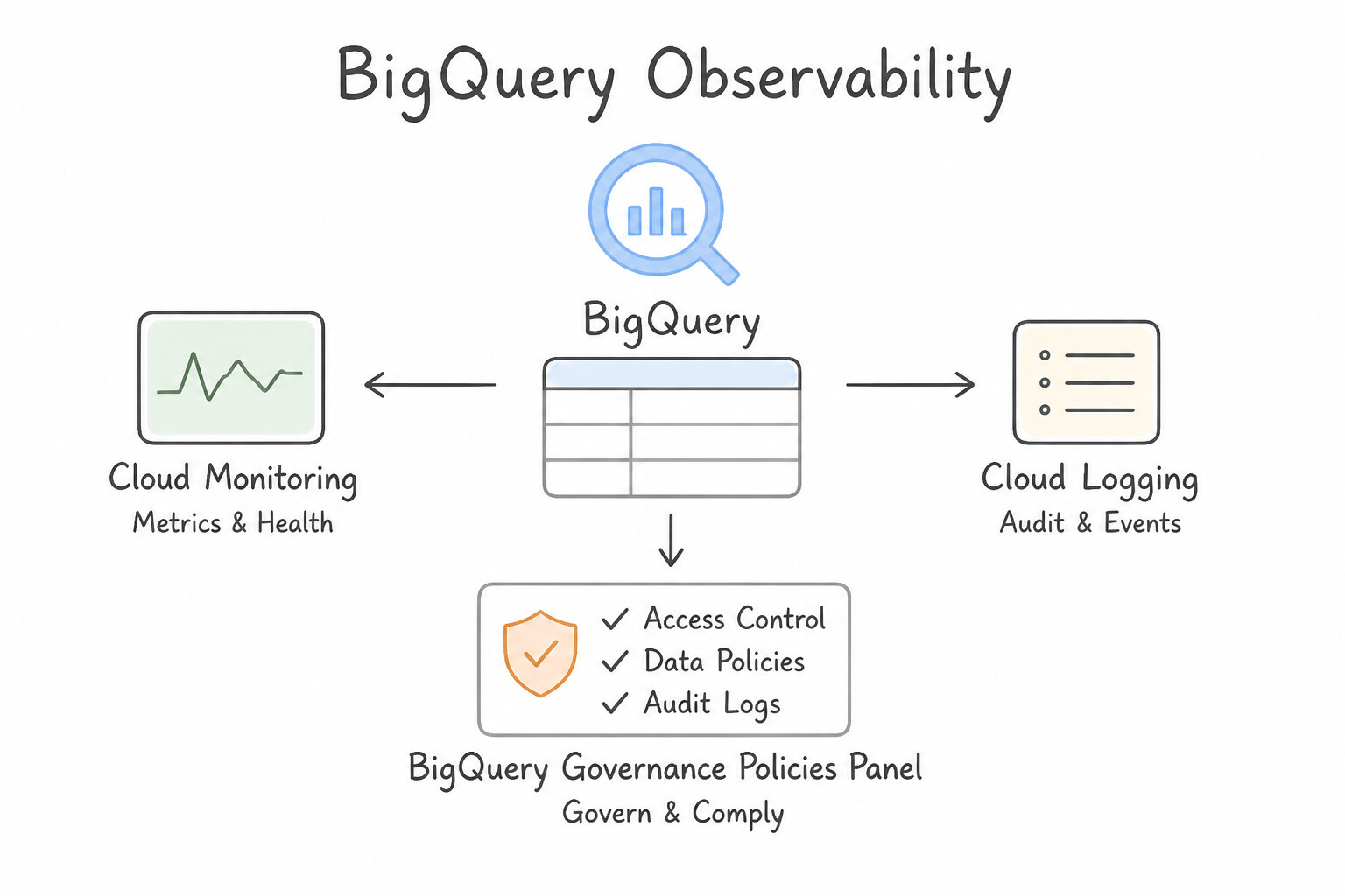
Know the exact observability tool for each Google Cloud data service:

• BigQuery Observability (Admin Panel + INFORMATION_SCHEMA):
• BigQuery Admin Panel (Monitoring / Resource Charts): Built-in visual console showing real-time and historical Slot Usage, Job Concurrency, Job Duration percentiles, and Error Rates broken down by Reservation and Project.
• INFORMATION_SCHEMA.JOBS_BY_PROJECT / JOBS_BY_ORGANIZATION: The authoritative SQL view for auditing every query's user_email, total_bytes_billed, total_slot_ms, referenced_tables, error_result, and job_stages over the past 180 days.
• INFORMATION_SCHEMA.RESERVATIONS_TIMELINE: Tracks per-minute slots_assigned, slots_max_assigned, and autoscale_current_slots to identify when reservations hit their ceiling.
• Dataflow Observability (Job Metrics + Cloud Monitoring):
• System Lag (dataflow.googleapis.com/job/system_lag): The primary SLI for streaming pipeline freshness—measures the maximum time an element has been waiting inside any stage of the pipeline.
• Data Watermark Age (data_watermark_age): Age of the most recent watermark (if growing linearly with wall-clock time, an upstream Pub/Sub partition is stuck or an unacknowledged message is blocking watermark progress!).
• Custom Beam Metrics (Metrics.counter(), Metrics.distribution()): Instrument business-level counters (e.g., malformed_records_count, dlp_api_latency_ms) inside your DoFn and export them automatically to Cloud Monitoring for alerting!
• Cloud Bigtable (Key Visualizer) & Cloud Dataproc (Component Gateway):
• Bigtable Key Visualizer: Generates a visual heatmap of read/write pressure across key ranges over time. A bright horizontal stripe indicates a single row key (or narrow prefix) receiving disproportionate traffic (hotspot); a diagonal bright line indicates a sequential timestamp key moving across tablets over time!
• Dataproc Component Gateway: Provides secure, authenticated one-click HTTPS access to the Spark History Server, YARN ResourceManager UI, and JupyterLab without opening SSH tunnels or public firewall ports.

Key Implementation Patterns

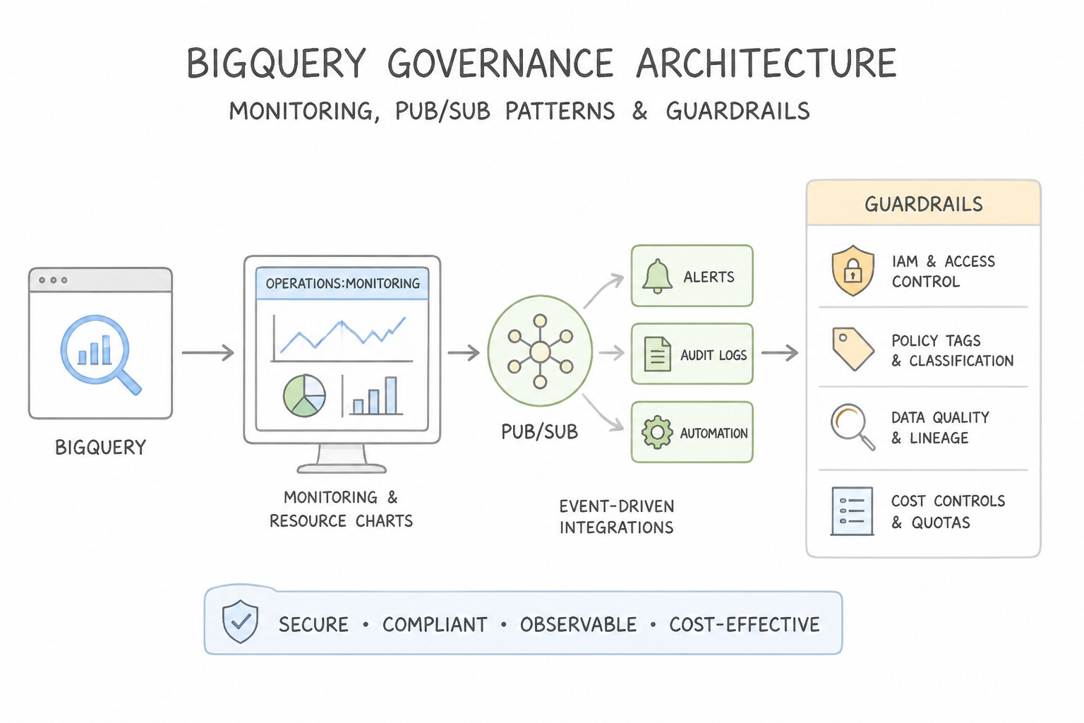
• Diagnosing BigQuery Performance Degradation: Use Use Cloud Monitoring to inspect the slot usage and concurrency metrics for the project during the affected time window. Performance degradation at specific times with unchanged queries suggests resource contention; checking slot usage metrics confirms if the system is constrained.
• Monitoring Pub/Sub Subscriber Backlog: Use Create an alert based on the 'subscription/oldest_unacked_message_age' metric. This metric directly measures the time latency (staleness) of the oldest message waiting to be processed. (Avoid alternative: This metric tracks the rate of incoming messages from publishers, not the subscriber backlog or latency.)
• Troubleshooting Dataflow Worker Failures: Use Inspect the Worker Logs in Cloud Logging to view exceptions thrown by your code. Worker Logs capture errors and exceptions directly from the code running on the worker instances. (Avoid alternative: Job Logs describe the service status, not the specific exceptions from your code.)

Key Takeaways (5.4a)

• Diagnose before solving: Always use monitoring metrics to confirm the root cause before scaling resources.
• Look for patterns: Performance issues occurring at specific times often indicate resource contention due to high concurrency.
• Understand Slots: BigQuery performance relies on 'slots'. Monitoring slot usage helps identify if you are hitting capacity limits.
• oldest_unacked_message_age is the primary metric for monitoring processing latency (staleness) in Pub/Sub.

Consideration 5.4b: Monitoring planned usage

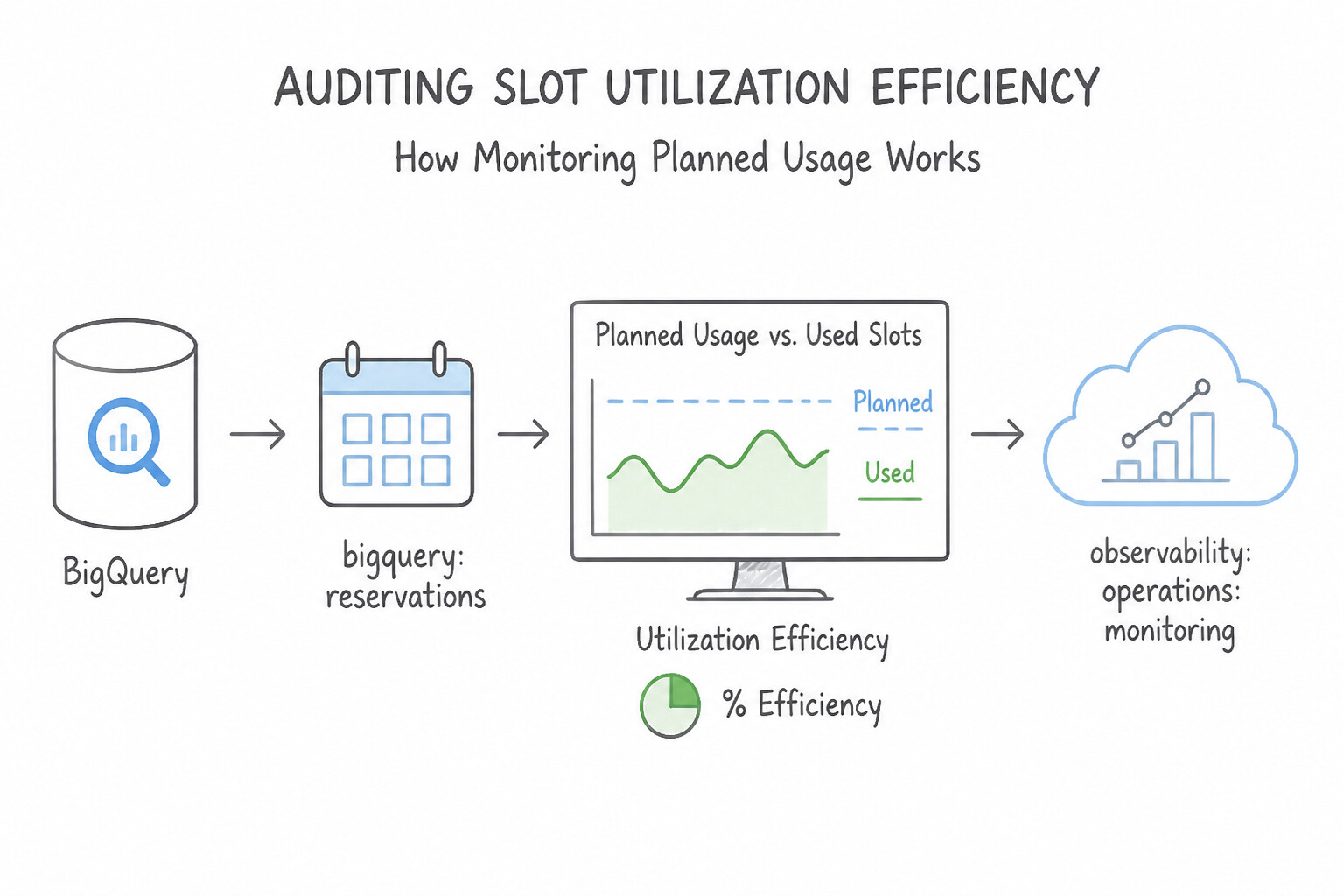
Proactively monitor capacity utilization against planned growth:

• Auditing Slot Utilization Efficiency:
• Divide a query's total_slot_ms by TIMESTAMP_DIFF(end_time, start_time, MILLISECOND) in INFORMATION_SCHEMA.JOBS_BY_ORGANIZATION to compute the average number of slots consumed.
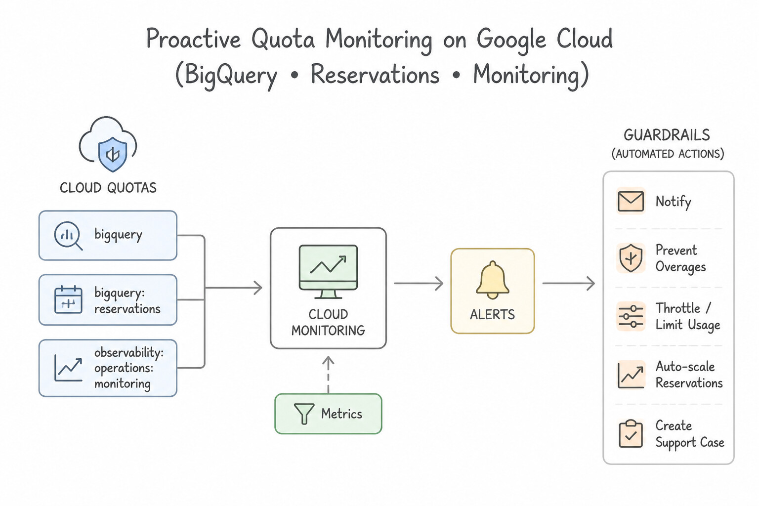
• Use the BigQuery Slot Estimator in the Admin Panel to model how raising or lowering baseline/autoscale slot caps impacts historical query queueing times (pending_units).
• Proactive Quota Monitoring (Cloud Quotas + Cloud Monitoring):
• Create Cloud Monitoring alerting policies on serviceruntime.googleapis.com/quota/allocation/usage and rate/net_usage to fire a PagerDuty/Slack notification when any project exceeds 80% of its Compute Engine CPU, IP address, or BigQuery API quota—before a production scale-up fails!

Key Implementation Patterns

• BigQuery Slot Utilization Monitoring: Use View the Slot Utilization chart in the BigQuery Admin panel to compare actual usage against the 2000 slot capacity. The BigQuery Admin Slot Utilization chart visualizes usage versus capacity, directly confirming if the 2000 slot limit is the bottleneck.
• Bigtable Node Scaling based on Storage: Use Add more nodes to the cluster. Bigtable SSD nodes should keep storage utilization below 70% for optimal performance; adding nodes distributes storage usage. (Avoid alternative: You cannot change storage type on an existing cluster, and HDD offers significantly lower performance than SSD.)
• Proactive Quota Management for Dataflow: Use Create an alert policy in Cloud Monitoring using the quota allocation usage metric. Set a threshold to notify you when usage approaches the limit. Use Cloud Monitoring to track the quota usage metric and alert you when it approaches the limit.

Key Takeaways (5.4b)

• BigQuery Slots represent compute capacity; a fixed reservation limits the maximum concurrent compute power.
• Slot Contention results in queuing and slower execution, not immediate errors.
• Use the BigQuery Admin panel or Cloud Monitoring to visualize slot usage versus capacity.
• Verify resource bottlenecks before purchasing additional capacity or optimizing individual queries.

Consideration 5.4c: Troubleshooting error messages, billing issues, and quotas

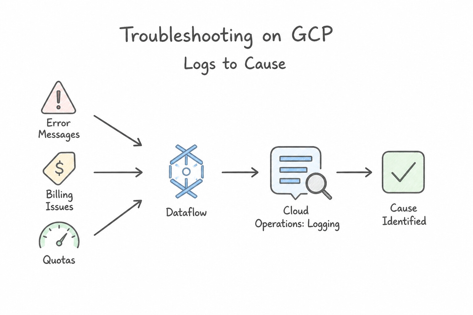
Memorize the root cause and exact fix for the top 6 PDE troubleshooting scenarios:

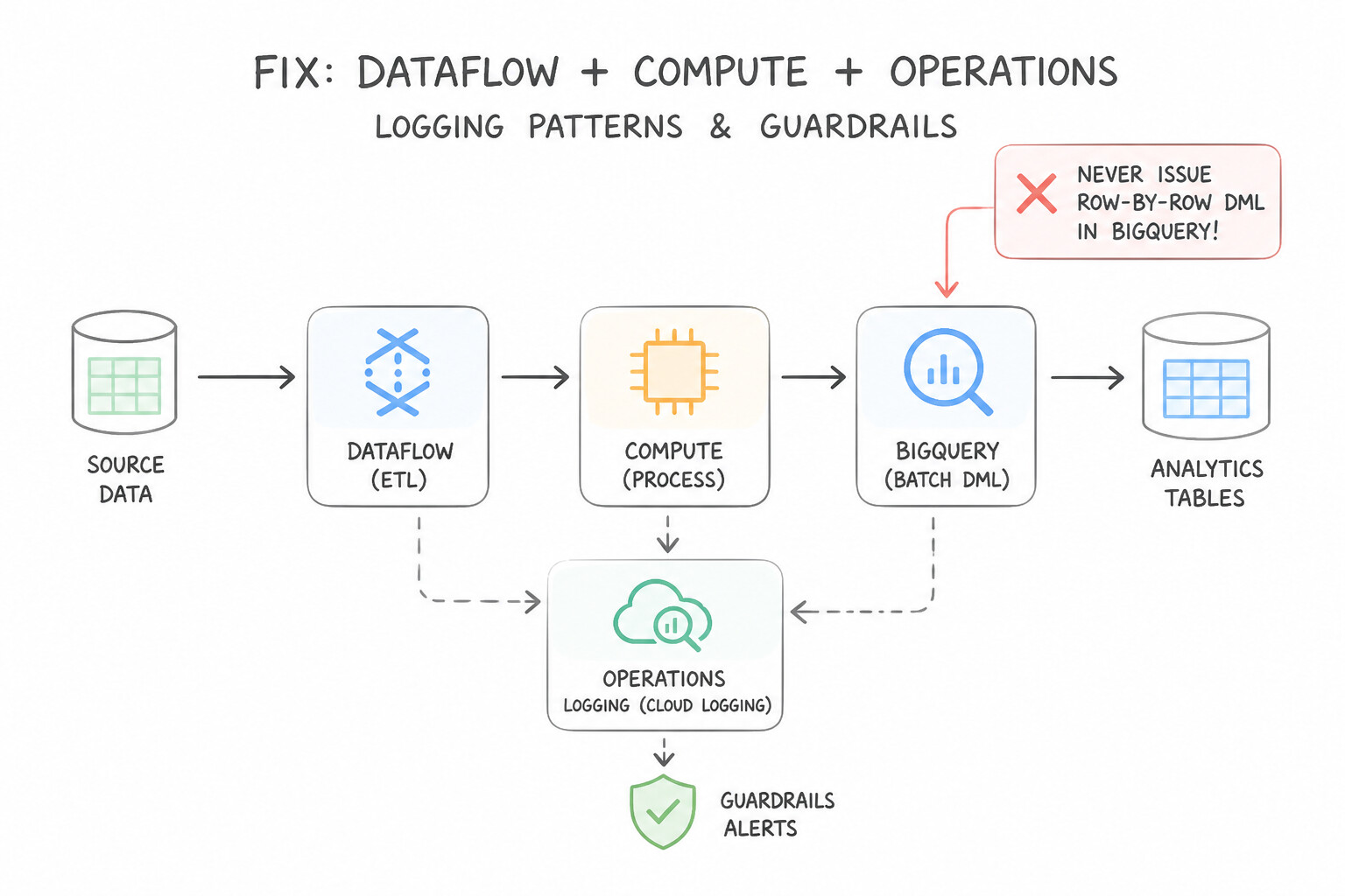
1. BigQuery rateLimitExceeded / quotaExceeded on Table DML or Table Metadata Updates:
2. Cause: Issuing thousands of single-row INSERT / UPDATE DML statements per minute from an application loop.
3. Fix: Never issue row-by-row DML in BigQuery! Batch DML updates into periodic bulk MERGE statements, or stream records via the BigQuery Storage Write API.
4. BigQuery Billing Spike Despite Partitioning (SELECT * or Function on Partition Column):
5. Cause: Analysts running SELECT * (scanning all 150 columns) or filtering with WHERE DATE(partition_ts) = '2026-10-13' in a way that prevents pruning, or querying without a partition filter.
6. Fix: Enable require_partition_filter = true, train/enforce explicit column projection, use Clustered columns, and set a project-level/user-level Custom Query Quota or maximum_bytes_billed.
7. Dataflow Worker OutOfMemoryError (OOM) vs. Straggler Tasks:
8. OOM Cause: Large un-splittable elements (e.g., a 1 GB gzipped CSV file—Note: gzip files cannot be split across workers by Dataflow, so a single worker must decompress the entire file in memory!), large unwindowed GroupByKey bags, or loading a massive Side Input into worker RAM.
9. OOM Fix: Use splittable formats (Avro or Parquet instead of .csv.gz), use highmem worker machine types or Dataflow Prime Vertical Autoscaling, and replace GroupByKey with Combine.perKey.
10. Dataproc / Spark ExecutorLostFailure (Exit code 137 / OOM) or Stage Stragglers:
11. Cause: Severe key skew during a Spark join or groupBy where one partition is 100x larger than the others.
12. Fix: Enable Spark Adaptive Query Execution (AQE — spark.sql.adaptive.enabled=true & spark.sql.adaptive.skewJoin.enabled=true), salt the skewed join key, or increase spark.executor.memory / spark.sql.shuffle.partitions.
13. Dataflow Job Fails to Scale Up (QUOTA_EXCEEDED on CPUs / Disks / IP Addresses):
14. Fix: Check Cloud Logging for the exact quota metric (CPUS, SSD_TOTAL_GB, or subnet IP_SPACE_EXHAUSTED), request a quota increase in Cloud Quotas, or enable Dataflow Streaming Engine / Shuffle Service (which dramatically reduces per-worker Persistent Disk and CPU requirements!).
15. Cloud Composer Tasks Fail with Zombie or AirflowTaskTimeout:
16. Cause: Heavy data processing inside the Airflow worker pod exhausted worker RAM (OOMKilled by GKE).
17. Fix: Offload processing to BigQuery/Dataflow/Dataproc, or run the task in an isolated KubernetesPodOperator with dedicated memory requests.

Key Implementation Patterns

• Dataflow Regional CPU Quota Exhaustion: Use Verify the Compute Engine resource quotas in the region and request an increase. Dataflow workers are Compute Engine VMs subject to regional resource quotas (like CPUs) that must be increased when exhausted. (Avoid alternative: Increasing the worker limit demands more resources, which worsens the existing quota exhaustion issue.)
• Troubleshooting 403 Access Denied in Dataproc: Use Grant the Storage Object Admin role to the VM Service Account used by the Dataproc cluster on the destination bucket. Dataproc jobs run on worker nodes that use the VM Service Account identity to access external resources like Cloud Storage.
• BigQuery Slot Exhaustion and Fair Scheduling: Use Switch the project to BigQuery Editions and create a reservation with baseline slots. On-demand slots are limited and best-effort; BigQuery Editions with Reservations provide guaranteed compute capacity. (Avoid alternative: Increasing concurrency quotas does not increase compute power (slots); queries will still wait if slots are full.)

Key Takeaways (5.4c)

• Dataflow workers are Compute Engine VMs that consume project quotas.
• "Quota exceeded" errors indicate hitting a resource limit (like CPUs or IP addresses), not a billing issue.
• Resource quotas are region-specific and must be monitored during autoscaling events.
• Resolving quota errors involves requesting a limit increase via the IAM & Admin console.

Consideration 5.4d: Managing workloads such as jobs, queries, and compute capacity (reservations)

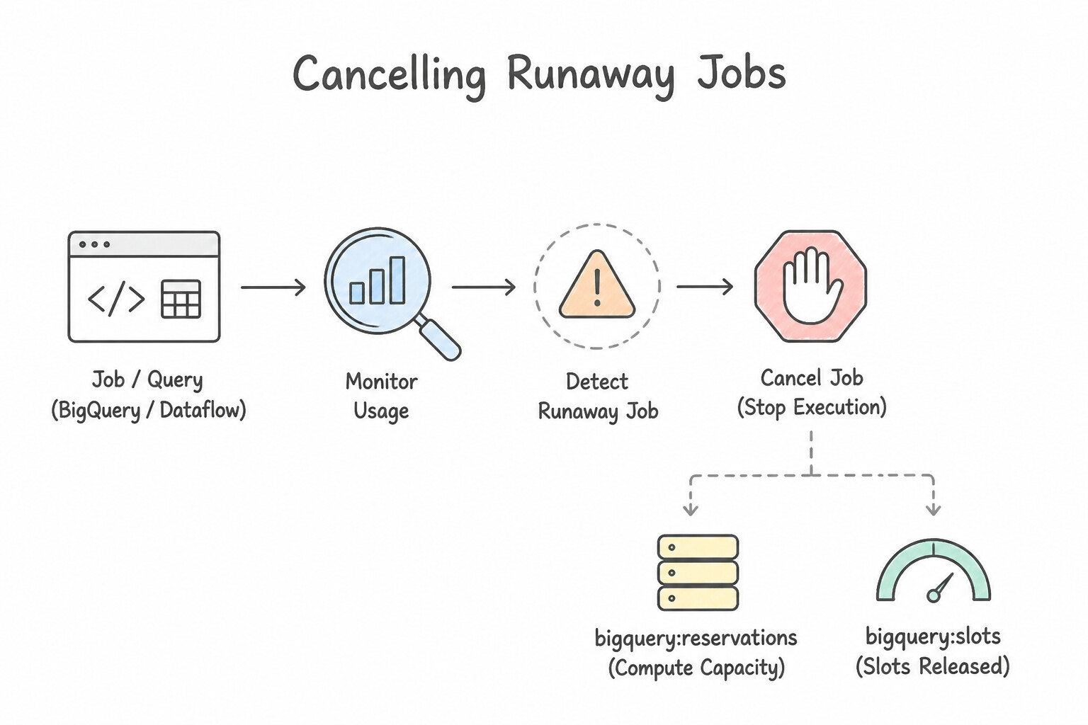
Act decisively when managing live production workloads:

• Cancelling Runaway Jobs:
• In BigQuery, identify a runaway query via INFORMATION_SCHEMA.JOBS_BY_PROJECT WHERE state = 'RUNNING' and terminate it immediately with CALL BQ.JOBS.CANCEL('project_id.us.job_id') or bq cancel <job_id>.
• In Dataflow, understand the three stop modes:
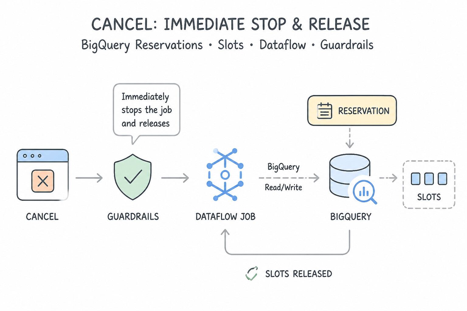
• Cancel: Immediately stops the job and releases VMs; in-flight buffered data is lost. Use only when a job is writing corrupted output or stuck in an unrecoverable state.
• Drain: Stops reading new data from unbounded sources (Pub/Sub), processes and flushes all in-flight buffered windows to sinks, and then shuts down cleanly with zero data loss.
• Update (--update): Replaces a running streaming job in-place while preserving window and watermark state.

Key Implementation Patterns

• Isolating Critical Workloads in BigQuery: Use Enable BigQuery Editions, create a dedicated reservation for the dashboards, and assign the dashboard project to this reservation. Reservations provide guaranteed compute capacity (slots) for specific projects, isolating critical workloads from noisy neighbors.
• Troubleshooting Dataflow OOM Errors: Use Configure the pipeline to use n1-highmem machine types for the workers. Since CPU usage is low but memory is causing crashes, switching to a high-memory machine type provides the necessary RAM to handle the workload. (Avoid alternative: Adding more workers helps with throughput but does not increase the memory available to an individual worker for processing large operations.)

Key Takeaways (5.4d)

• Resource Isolation: Use BigQuery Reservations to isolate critical workloads (like dashboards) from ad-hoc or batch workloads.
• Guaranteed Capacity: Reservations ensure a baseline of performance by dedicating slots to specific projects.
• Assignments: You must assign a project to a reservation for it to utilize the reserved slots; otherwise, it uses the default pool.
• Analyze Error Types: Java heap space errors specifically point to RAM exhaustion.

Quick Decision Cheat Sheet (Subsection 5.4)

Further Reading (Subsection 5.4)

• Introduction to BigQuery Slots — Explains the concept of slots as virtual CPUs and how they are used to process queries.
• Monitoring BigQuery using Cloud Monitoring — Details the available metrics in Cloud Monitoring, including slot allocation and concurrency.
• Monitoring Pub/Sub — Refer to the 'Metric types' table, specifically the 'subscription/oldest_unacked_message_age' row, which explains that it measures the age of the oldest unacknowledged message.
• Using Cloud Logging with Dataflow — Provides an overview of the different log types (Job, Worker, Startup) and how to access them.
• Introduction to Reservations — Provides an overview of how slots, reservations, and assignments work in BigQuery Editions.
• Monitoring BigQuery Reservations — Explains how to use the Administrative charts to view slot usage and troubleshoot capacity issues.

Subsection 5.5: Maintaining awareness of failures and mitigating impact

Section 5: Maintaining and Automating Data Workloads

The Big Picture

Hardware fails, zones experience power events, upstream teams deploy buggy code that corrupts a production table, and network links drop packets. Subsection 5.5 is the ultimate test of resilience engineering—designing data systems that survive infrastructure and human failures without breaching business SLAs:

1. Regional HA vs. Cross-Region Disaster Recovery (5.5b, 5.5d): Students frequently confuse High Availability (HA within a single region across zones) with Disaster Recovery (DR across two separate geographic regions)!
2. In Cloud SQL, enabling High Availability (Regional HA) provisions a synchronous standby instance in a second zone of the same region (via Regional Persistent Disk), providing automatic failover with RPO = 0 if the primary zone fails. However, if the entire region goes down, a regional standby cannot help—you must also configure a Cross-Region Read Replica and promote it during a regional outage!
3. In Memorystore for Redis, the Basic Tier is a single standalone node (any maintenance or failure wipes the cache completely); only the Standard Tier (or Memorystore for Redis Cluster with multi-zone replicas) provides cross-zone replication and automatic failover.
4. Recovering from Human/Code Data Corruption (5.5c): Hardware replication faithfully replicates a human mistake (DELETE FROM prod.orders WHERE 1=1 or a buggy ETL overwrite) to every replica in milliseconds! Recovering from logical data corruption requires BigQuery Time Travel (FOR SYSTEM_TIME AS OF), BigQuery Table Snapshots, Cloud Storage Object Versioning (with noncurrent version restoration), or Cloud SQL Point-in-Time Recovery (PITR) backed by binary logs / WAL!

Consideration 5.5a: Designing system for fault tolerance and managing restarts

Distinguish transient infrastructure faults from permanent data faults, and design clean restart workflows:

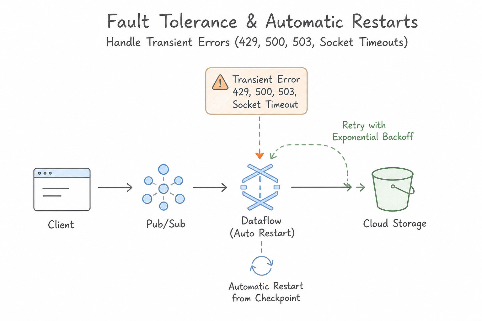
• Transient Errors (HTTP 429, 500, 503, Socket Timeouts):
• Mitigate with truncated exponential backoff with random jitter (wait = min(max_backoff, base * 2^attempt + random_jitter)). Jitter is essential so 500 workers retrying after a brief downstream outage do not hammer the target API at the exact same millisecond (thundering herd).
• In Apache Beam on Dataflow, failed work bundles are automatically retried (up to 4 times in batch, indefinitely in streaming to guarantee data completeness—which is why permanent parsing exceptions must be caught and routed to a Dead-Letter Queue so they don't block the streaming job forever!).
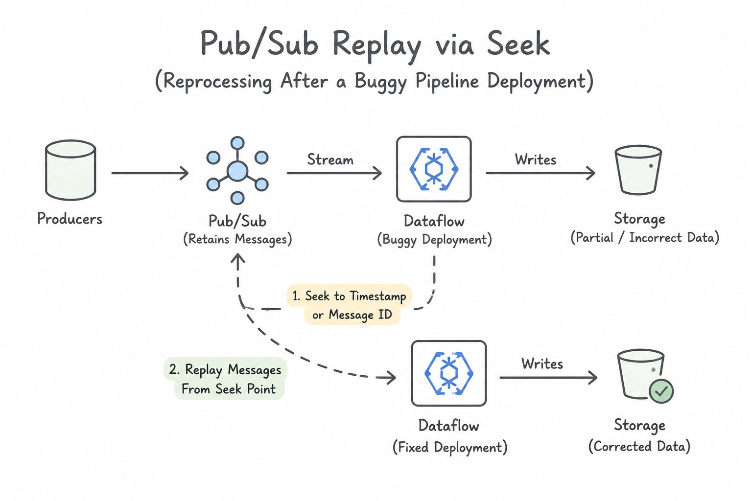
• Pub/Sub Replay via Seek (Reprocessing After a Buggy Pipeline Deployment):
• If a buggy Dataflow deployment ran for 3 hours writing corrupted logic to a sink, how do you reprocess the last 3 hours of Pub/Sub messages without asking upstream producers to resend them?
• Configure Retain Acknowledged Messages (retain_acked_messages = true) on the Pub/Sub subscription (or take periodic Pub/Sub Snapshots before deployments), deploy the fixed pipeline, and issue a gcloud pubsub subscriptions seek command to rewind the subscription cursor back to a timestamp 3 hours ago (or to the pre-deployment Snapshot)!

Key Implementation Patterns

• Handling Malformed Data in Streaming Pipelines: Use Update the pipeline code to use a side output that routes invalid messages to a separate storage location. Side outputs allow you to route bad data to a Dead Letter Queue without stopping the main pipeline. (Avoid alternative: Draining stops the pipeline entirely, which disrupts processing of valid messages.)
• Recovering from Logical Errors in Consumers: Use Use the Seek feature on the subscription to reset the cursor to a timestamp from four hours ago. The Seek feature allows you to replay previously acknowledged messages from a specific point in time. (Avoid alternative: New subscriptions only capture messages published after the moment of creation.)
• Orchestration Resilience for Flaky APIs: Use Configure the retries and retry_delay parameters in the PythonOperator definition. Airflow operators natively support retries using the retries and retry_delay parameters, which is the standard way to handle transient errors.

Key Takeaways (5.5a)

• Streaming pipelines must be designed to handle bad data gracefully to avoid indefinite retries or stalls.
• The Side Output pattern in Apache Beam is the primary method for creating Dead Letter Queues (DLQs) in Dataflow.
• Never drop bad data silently; preserve it in a separate storage system for analysis and potential replay.
• Seek allows you to replay messages in Pub/Sub by resetting the subscription cursor to a past timestamp or snapshot.

Consideration 5.5b: Running jobs in multiple regions or zones

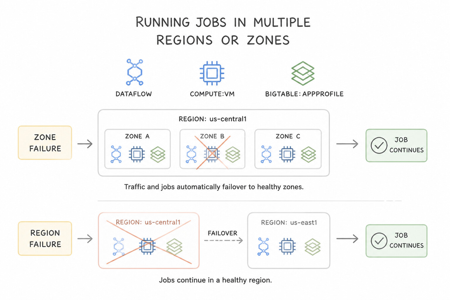
Design compute and storage topologies that survive zone and region failures:

• Zone Failures vs. Region Failures:
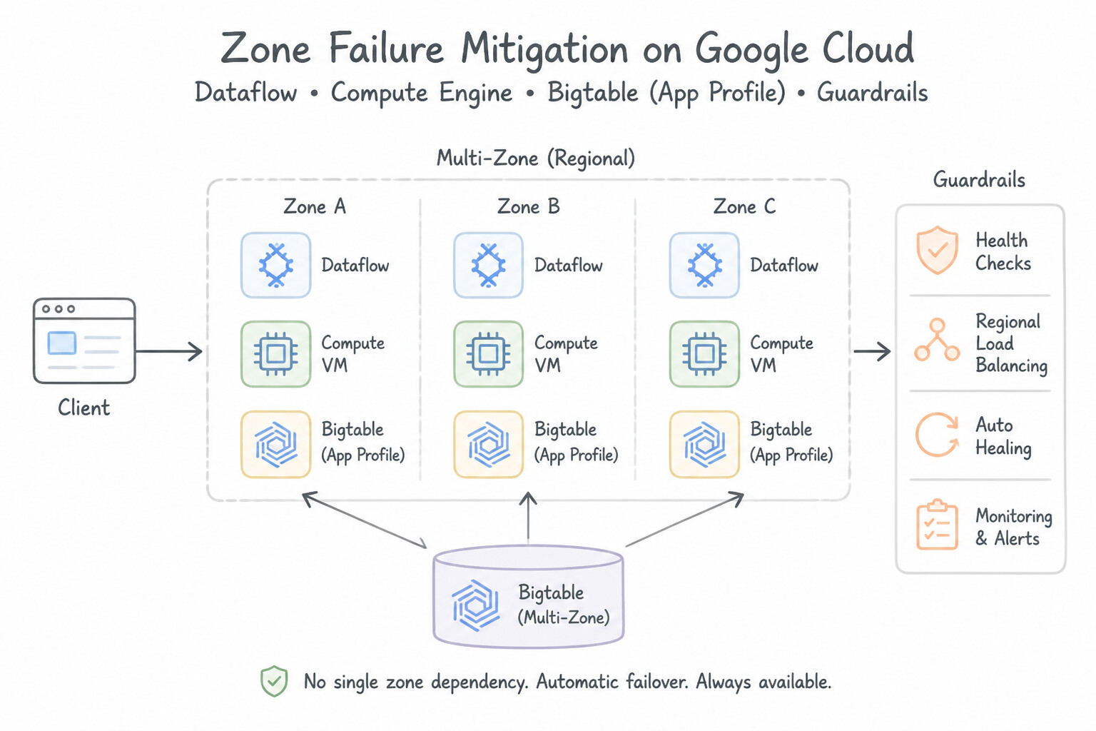
• Zone Failure Mitigation: When you submit a Dataflow job or create a Dataproc cluster with Auto Zone placement in a region (e.g., us-central1) and use a Regional Cloud Storage bucket (or Streaming Engine), Google Cloud distributes resources across multiple availability zones within that region.
• Region Failure Mitigation (Cross-Region DR):
• For Cloud Storage, use a Dual-Region (with Turbo Replication for a 15-minute RPO SLA) or Multi-Region bucket.
• For BigQuery, enable Cross-Region Dataset Replication (ALTER SCHEMA ... ADD REPLICA) to a secondary region; if the primary region fails, promote the secondary dataset replica to primary with zero application SQL changes.
• For Dataflow / Dataproc, keep pipeline templates (Dataflow Flex Templates in multi-region Artifact Registry) and orchestration DAGs (Cloud Composer snapshots in dual-region GCS) ready to launch in the secondary region against the replicated storage.

Key Implementation Patterns

• Dataflow Zonal Availability: Use Remove the --workerZone flag and use the --workerRegion flag to specify the target region. Switching from a specific zone to a region allows Dataflow to automatically place workers in a healthy zone. (Avoid alternative: Code-level exception handling cannot resolve infrastructure outages preventing worker startup.)
• Cloud Bigtable Automatic Failover: Use Configure the App Profile to use multi-cluster routing to any cluster. Multi-cluster routing automatically routes traffic to the nearest healthy cluster, ensuring high availability during outages. (Avoid alternative: Single-cluster routing pins traffic to one cluster and does not support automatic failover.)
• Cloud Spanner Global Availability: Use Create a Multi-Region instance configuration that spans three distinct regions. A Multi-Region configuration provides 99.999% availability and survives the loss of an entire region. (Avoid alternative: A Regional configuration protects against zone failures (99.99% availability) but not region failures.)

Key Takeaways (5.5b)

• Avoid pinning managed services to specific zones unless necessary for data locality or latency.
• Use regional parameters (like --workerRegion) to allow Google Cloud to manage zonal placement and availability.
• Hardcoded zonal constraints create Single Points of Failure (SPOF).
• Cloud Bigtable App Profiles control how applications connect to clusters and handle routing.

Consideration 5.5c: Preparing for data corruption and missing data

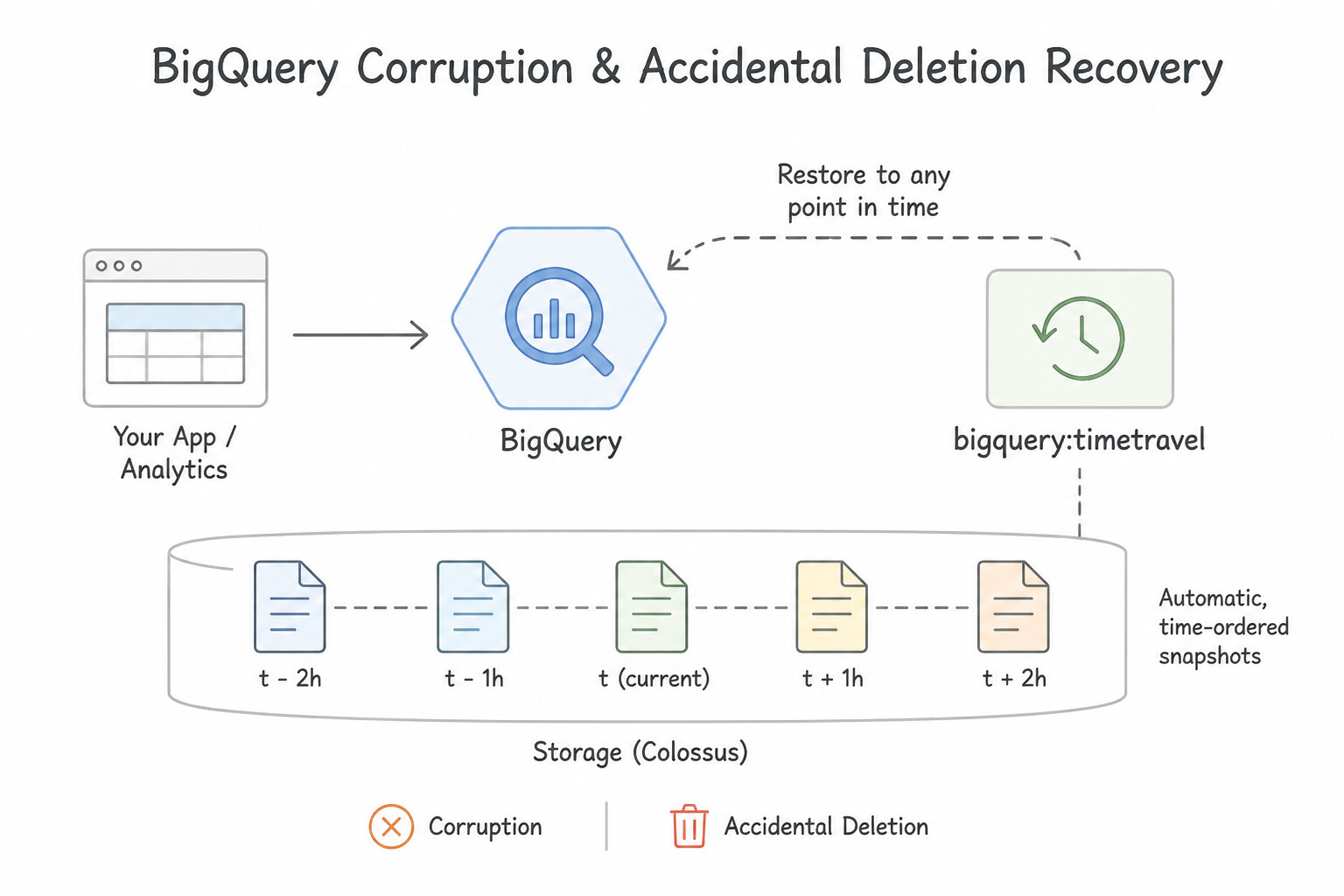
Memorize the exact recovery mechanism when bad code or human error corrupts or deletes data:

• BigQuery Corruption / Accidental Deletion Recovery:
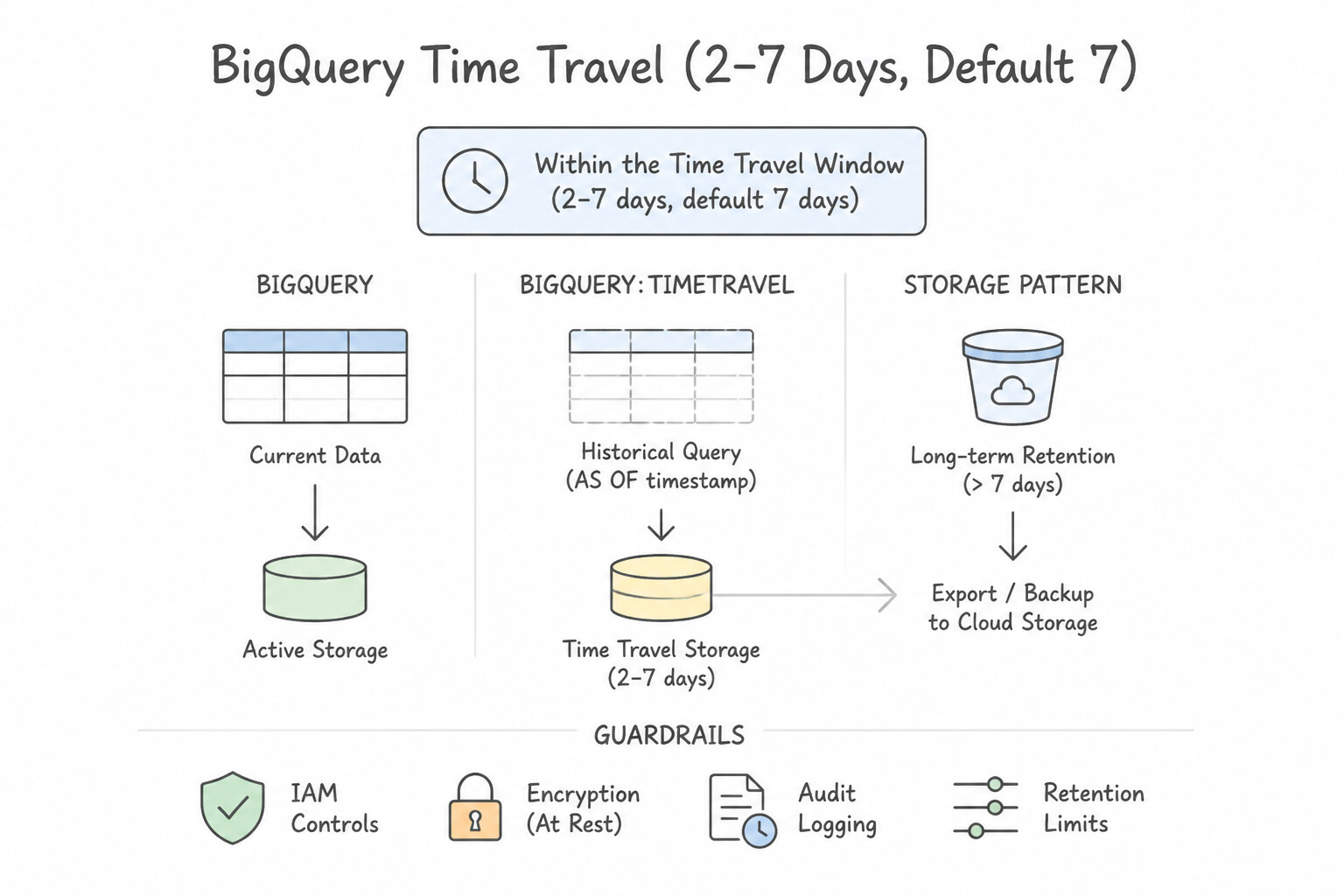
• Within the Time Travel Window (2–7 days, default 7 days):
• If a table's rows were corrupted or overwritten by bad DML 6 hours ago: CREATE OR REPLACE TABLE prod.orders AS SELECT * FROM prod.orders FOR SYSTEM_TIME AS OF TIMESTAMP_SUB(CURRENT_TIMESTAMP(), INTERVAL 6 HOUR).
• If the table itself was dropped (DROP TABLE prod.orders) 6 hours ago: run bq cp prod.orders@-21600000 prod.orders_restored (using the relative millisecond offset decorator @-<ms> or absolute epoch timestamp @<ms>)!
• Beyond 7 Days: Restore from scheduled BigQuery Table Snapshots (or within the 7-day post-Time-Travel Fail-safe window via Google Cloud Support).
• Cloud Storage Corruption / Accidental Overwrite Recovery:
• Object Versioning: Retains a noncurrent generation every time an object is overwritten or deleted. To recover from a buggy pipeline that overwrote gs://lake/config.json, copy the previous object#generation back to live (and use Object Lifecycle Management Delete after NumNewerVersions: 3 or DaysSinceNoncurrentTime: 30 to bound versioning storage costs).
• Soft Delete Policy (Default 7 Days, up to 90 Days): Protects deleted objects from permanent loss by holding them in a soft-deleted state where they can be restored even if Object Versioning was not enabled!
• Cloud SQL Corruption Recovery:
• Enable Automated Backups + Point-in-Time Recovery (PITR / Binary Logging / Write-Ahead Logs) to clone/restore the database to the exact second before the accidental DROP TABLE or bad UPDATE occurred.

Key Implementation Patterns

• Recovering from Accidental DML Operations: Use Run a query using the FOR SYSTEM_TIME AS OF clause with a timestamp from one hour ago. Overwrite the table with the query results. BigQuery Time Travel allows immediate querying of historical data from the last 7 days using SQL syntax.
• Protection Against Accidental Object Deletion: Use Enable Object Versioning on the Cloud Storage bucket. Object Versioning retains a history of object modifications, allowing you to restore previous versions if a file is overwritten or deleted. (Avoid alternative: Retention Policies prevent modification entirely for a set time, which is inflexible for updates, whereas Versioning allows updates but keeps a backup.)
• Handling Poison Pill Records in Streaming: Use Modify your DoFn to use a try-catch block that captures exceptions and directs malformed records to a side output. Use a try-catch block and side outputs to separate bad records (Dead Letter Queue) from valid data without stopping the pipeline.

Key Takeaways (5.5c)

• BigQuery Time Travel retains a 7-day history of data changes by default.
• Use the FOR SYSTEM_TIME AS OF SQL clause to query historical data immediately.
• Time Travel is the fastest way to recover from accidental data corruption or deletion within the 7-day window.
• Table snapshots allow for longer retention but must be created explicitly before the corruption occurs.

Consideration 5.5d: Data replication and failover (e.g., Cloud SQL, Redis clusters)

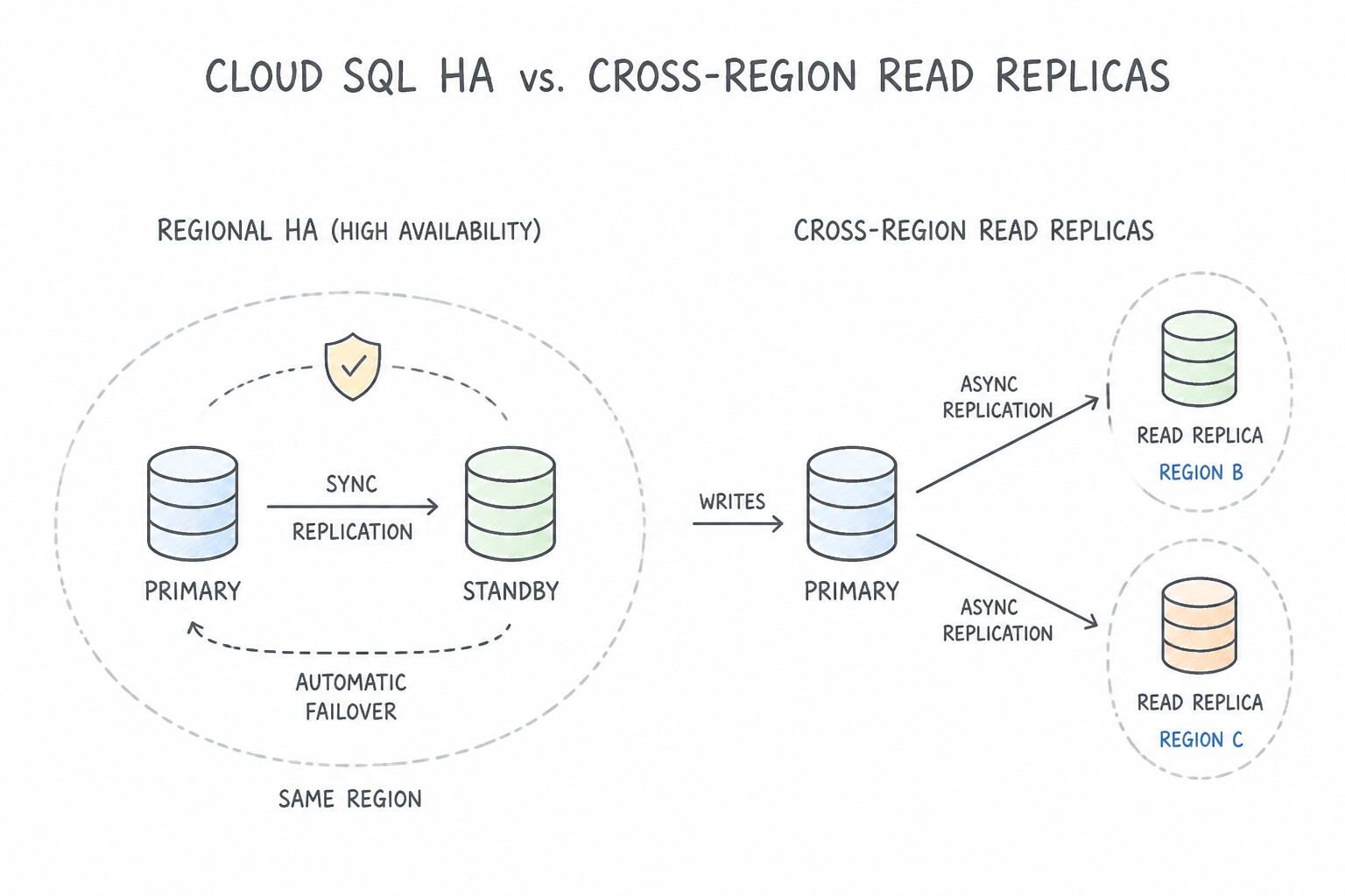
Distinguish the exact failover architectures of Google Cloud's operational data stores:

• Cloud SQL High Availability (Regional HA) vs. Cross-Region Read Replicas:
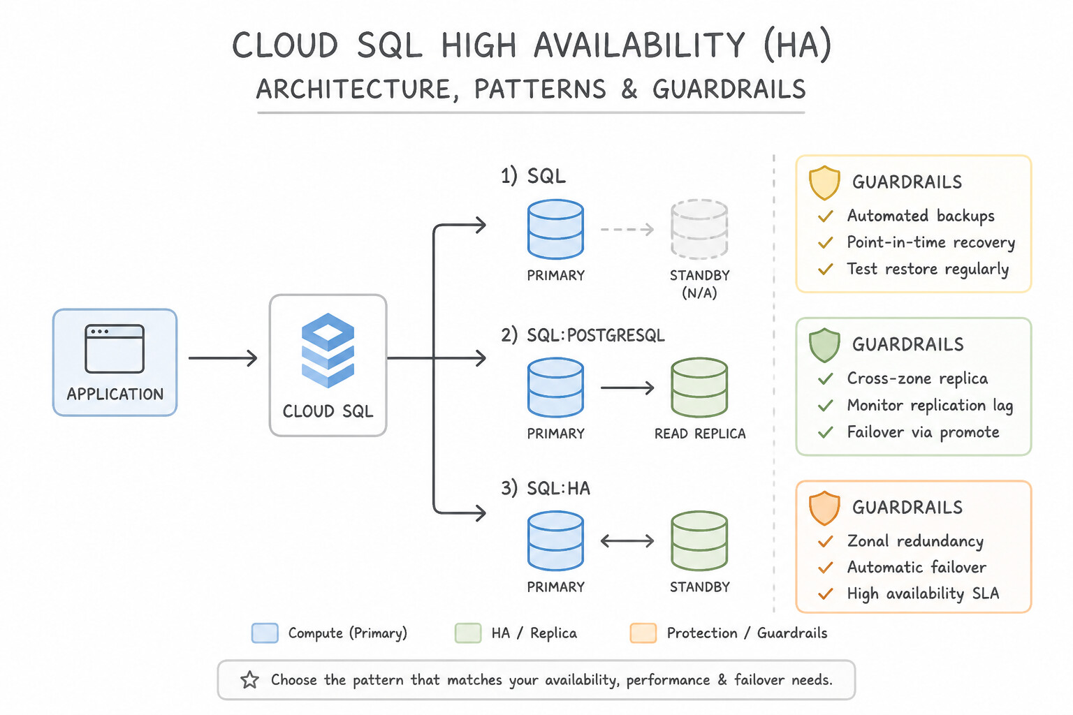
• Cloud SQL High Availability (HA): Protects against Zone Failure within a single region. Uses synchronous block-level replication via Regional Persistent Disks to a standby VM in another zone of the same region. When the primary zone or instance fails, Cloud SQL automatically fails over to the standby in ~60 seconds with RPO = 0 (zero data loss), keeping the same IP address.
• Cloud SQL Cross-Region Read Replica: Protects against Full Regional Outage (and offloads read traffic). Uses asynchronous replication to a second region. If the primary region goes dark, you manually (or via automated script/Database Migration Service DR) promote the Cross-Region Read Replica to a standalone primary instance (RPO > 0 by seconds of replication lag).
• Deletion Protection (deletion_protection = true) & Maintenance Windows: Enable deletion_protection on production Cloud SQL and BigQuery tables so accidental gcloud sql instances delete calls are blocked; configure Maintenance Windows during off-peak hours.
• Memorystore for Redis (Basic vs. Standard Tier & Redis Cluster):
• Basic Tier: Single node, zero replication—any zone failure or maintenance restarts the node and flushes all cached keys (cold cache!).
• Standard Tier (and Memorystore for Redis Cluster with replicas): Provisions primary and replica nodes across multiple availability zones with automatic failover (usually <30 seconds) and optional RDB Snapshot / AOF persistence to survive node failures without cache-stampeding your backend database.
• Cloud Bigtable Multi-Cluster Automatic Failover:
• Configure a Bigtable instance with 2+ clusters in different zones or regions, and point your application to an App Profile configured with Multi-Cluster Routing. If Cluster 1's zone or region fails, Bigtable automatically routes traffic to Cluster 2 without manual intervention!

Key Implementation Patterns

• Cloud SQL High Availability Configuration: Use Enable the High availability (HA) configuration on the instance. High Availability (HA) creates a standby instance with synchronous replication and enables automatic failover if the primary zone fails. (Avoid alternative: Read replicas are for scaling reads and require manual promotion for failover; they do not provide automatic failover by default.)
• Bigtable Multi-Cluster Routing: Use Configure the application profile to use multi-cluster routing. Multi-cluster routing enables automatic failover to the nearest available cluster. (Avoid alternative: Single-cluster routing isolates traffic to one cluster and does not fail over automatically.)
• Cloud Memorystore for Redis Tier Selection: Use Upgrade the Cloud Memorystore instance to the Standard Tier. The Standard Tier automatically provisions a standby node in a different zone and handles automatic failover. (Avoid alternative: Persistence saves data to disk but does not provide a standby node or automatic failover for high availability.)

Key Takeaways (5.5d)

• High Availability (HA) in Cloud SQL provides automatic failover to a standby instance in a different zone.
• HA uses synchronous replication to ensure zero data loss for committed transactions during a failover.
• Read replicas are primarily for scaling read operations and typically use asynchronous replication.
• Backups are used for disaster recovery (restoring lost data), not for real-time failover.

Quick Decision Cheat Sheet (Subsection 5.5)

Further Reading (Subsection 5.5)

• Dataflow patterns - Handling bad data — Discusses patterns for robust pipelines, including handling exceptions and bad data using side outputs.
• Replaying messages (Seek) — Documentation on how to use the Seek feature to replay acknowledged messages by seeking to a timestamp or a snapshot.
• airflow.models.baseoperator &mdash; Airflow Documentation — Documentation for the BaseOperator class, which lists the 'retries' and 'retry_delay' arguments available to all operators.
• Google Cloud Composer: Writing DAGs — General guide on writing DAGs in Cloud Composer, covering best practices for task definition.
• Specifying a region for workers — Documentation explaining how to use the --workerRegion flag to allow the Dataflow service to automatically select the best zone for workers.
• Configuring App Profiles — Documentation explaining how App Profiles work, including the differences between single-cluster and multi-cluster routing policies.

Book TOC · Previous · Chapter 5 of 6 · Next